1  KKT Worked Examples

Author

Affiliation

Enrico Bertolazzi

University of Trento, Department of Industrial Engineering

1.1 Example 1: Detailed Example of Constrained Minimization

In this example, we will minimize the function

\begin{aligned} \text{minimize:}\quad & f(x, y) = x + y, \\ \text{subject to the constraint:}\quad & h(x, y) = x^2 + y^2 - 1 = 0, \end{aligned}

where h(x, y) = 0 describes a unit circle. We will approach this problem using two methods:

1. Parametrization with x = \cos(t) and y = \sin(t).
2. Lagrange Multipliers.

Parametric Solution

The constraint h(x, y) = x^2 + y^2 - 1 represents a unit circle. We can parametrize the constraint as:

x(t) = \cos(t), \quad y(t) = \sin(t), \quad t \in [0, 2\pi].

Substituting the parametrization into the objective function yields:

f(\cos(t), \sin(t)) = \cos(t) + \sin(t).

To find the critical points, we can differentiate this parametric function and analyze it:

Critical Points

The maximum and minimum values of f can be found by solving for t:

• The function f(\cos(t), \sin(t)) achieves its extrema when:

\frac{\mathrm{d}}{\mathrm{d}t} (\cos(t) + \sin(t)) = -\sin(t) + \cos(t) = 0.

This gives us:

\sin(t) = \cos(t) \quad \Rightarrow \quad t = \frac{\pi}{4} + k\pi, \, k \in \mathbb{Z}.

Function Values

Evaluating the function at these points:

• At t = \frac{5\pi}{4} (minimum):

\left. \begin{aligned} x &= \cos\left(\frac{5\pi}{4}\right) = -\frac{\sqrt{2}}{2}, \\ y &= \sin\left(\frac{5\pi}{4}\right) = -\frac{\sqrt{2}}{2}, \end{aligned} \right\} \quad \implies\quad f(x, y) = -\sqrt{2}.

• At t = \frac{\pi}{4} (maximum):

\left. \begin{aligned} x &= \cos\left(\frac{\pi}{4}\right) = \frac{\sqrt{2}}{2}, \\ y &= \sin\left(\frac{\pi}{4}\right) = \frac{\sqrt{2}}{2}, \end{aligned} \right\} \quad\implies\quad f(x, y) = \sqrt{2}.

Visualization

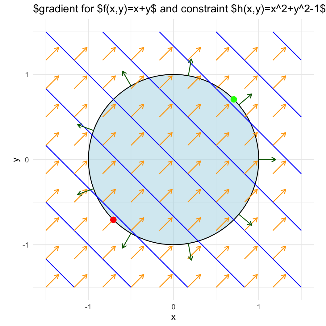
Let’s visualize the unit circle and the level sets of the objective function.

Figure 1.1: Objective level sets, gradient field, and the unit-circle constraint.

The plot illustrates that the minimum and maximum points occur where the gradient vector field of the function f(x, y) = x + y is aligned with the normal vectors of the constraint curve h(x, y) = x^2 + y^2-1. This alignment indicates that the gradient is parallel to the constraint’s normal, satisfying the first order necessary condition.

Lagrange Multipliers Method

Now, we will apply the method of Lagrange multipliers to our constrained optimization problem. We define the Lagrangian as follows:

\mathcal{L}(x, y, \lambda) = f(x, y) - \lambda h(x, y) = x + y - \lambda (x^2 + y^2 - 1).

First-Order Conditions

To find the extrema, we take the gradients of the Lagrangian with respect to x, y, and \lambda. This leads to the first-order conditions:

1. For x: \nabla_x \mathcal{L} = 1 - 2\lambda x = 0 \quad \Rightarrow \quad \lambda = \frac{1}{2x}.

2. For y: \nabla_y \mathcal{L} = 1 - 2\lambda y = 0 \quad \Rightarrow \quad \lambda = \frac{1}{2y}.

3. The constraint condition: h(x, y) = x^2 + y^2 - 1 = 0.

Solving the nonlinear system

Setting the two expressions for \lambda equal gives us:

\frac{1}{2x} = \frac{1}{2y} \quad \Rightarrow \quad x = y.

Next, substituting x = y into the constraint:

2x^2 = 1 \quad \Rightarrow \quad x = \pm \frac{1}{\sqrt{2}} \quad \Rightarrow \quad y = \pm \frac{1}{\sqrt{2}}.

Second-Order Conditions

To determine whether the critical points are minima or maxima, we need to evaluate the second-order conditions.

1. Second-Order Necessary Condition: The Hessian of the Lagrangian, \nabla_{(x,y)}^2 \mathcal{L}(x, y, \lambda), must be positive semidefinite in the null space of the constraint gradients.

2. Second-Order Sufficient Condition: The Hessian of the Lagrangian, \nabla_{(x,y)}^2 \mathcal{L}(x, y, \lambda), must be positive definite in the null space of the constraint gradients.

Computing the Hessian

The Hessian matrix of the Lagrangian with respect to x and y is given by:

\nabla^2 \mathcal{L}(x, y, \lambda) = \begin{bmatrix} \frac{\partial^2 \mathcal{L}}{\partial x^2} & \frac{\partial^2 \mathcal{L}}{\partial x \partial y} \\[0.5em] \frac{\partial^2 \mathcal{L}}{\partial y \partial x} & \frac{\partial^2 \mathcal{L}}{\partial y^2} \end{bmatrix} = \begin{bmatrix} -2\lambda & 0 \\ 0 & -2\lambda \end{bmatrix}.

Kernel of the Constraint

The kernel of the constraint

h(x, y) = 0

consists of the vectors \bm{z} that satisfy

\nabla h(x, y) \cdot \bm{z} = 0.

The gradient of the constraint is:

\nabla h(x, y) = [2x, 2y]

and it is easy to verify that the kernel of the constraint gradient can be spanned by vector \bm{z} = \begin{pmatrix} -y \\ x \end{pmatrix}

Check qualification

The equality-constraint gradient is nonzero at both candidates, hence LICQ holds.

Evaluating the Hessian at Critical Points

1. At point (x^\star,y^\star)=\left(-\frac{1}{\sqrt{2}}, -\frac{1}{\sqrt{2}}\right) the multiplier \lambda = -\frac{1}{\sqrt{2}}. The kernel of h(x,y) is spanned by \bm{z} = t \begin{pmatrix} y^\star\\-x^\star\end{pmatrix} = \frac{t}{\sqrt{2}} \begin{pmatrix} -1\\1\end{pmatrix} \in\ker\!\left(\nabla h(x^\star,y^\star)^\top\right)

   Thus the Hessian and second order condition becomes: \begin{aligned} \nabla^2_{(x,y)} \mathcal{L} & = \sqrt{2}\,I, \qquad \bm{z}^{\top} \nabla^2_{(x,y)} \mathcal{L} \bm{z}\quad\implies \\[0.5em] & \frac{t^2}{2} \begin{bmatrix}1 & -1\end{bmatrix} \left(\sqrt{2}\,I\right) \begin{bmatrix}1\\-1\end{bmatrix} =\sqrt{2}\,t^2 > 0, \end{aligned} for all t\neq 0. Therefore, this point is a strict local minimum.

2. At point (x^\star,y^\star)=\left(\frac{1}{\sqrt{2}},\frac{1}{\sqrt{2}}\right) the multiplier \lambda = \frac{1}{\sqrt{2}}.

   Thus the Hessian and second order condition becomes: \begin{aligned} \nabla^2_{(x,y)} \mathcal{L} & = -\sqrt{2}\,I, \qquad \bm{z}^{\top} \nabla^2_{(x,y)} \mathcal{L} \bm{z}\quad\implies \\[0.5em] & \frac{t^2}{2} \begin{bmatrix}1 & -1\end{bmatrix} \left(-\sqrt{2}\,I\right) \begin{bmatrix}1\\-1\end{bmatrix} =-\sqrt{2}\,t^2 < 0,\qquad \forall t\neq 0 \end{aligned} Therefore, this point is a strict local maximum.

Conclusion

Both methods yield the same results:

• The minimum occurs at \left(-\frac{1}{\sqrt{2}}, -\frac{1}{\sqrt{2}}\right) with f(x, y) = -\sqrt{2}.
• The maximum occurs at \left(\frac{1}{\sqrt{2}}, \frac{1}{\sqrt{2}}\right) with f(x, y) = \sqrt{2}.

1.2 Example 2: Detailed Example of KKT

In this example, we will minimize the function

\begin{aligned} \text{minimize:}\quad & f(x, y, z ) = x^2 + y + z, \\ \text{equality constraint:}\quad & x+y^2+z^2=1, \\ \text{and inequalities:}\quad & z\leq 1, \quad x \geq 0, \end{aligned}

Rewriting in Standard Form

We can rewrite the problem in a more standard form:

\begin{aligned} \text{minimize:}\quad & f(x, y, z ) = x^2 + y + z, \\ \text{equality constraint:}\quad & h(x,y,z) = x+y^2+z^2-1 = 0, \\ \text{and inequalities:}\quad & g_1(x,y,z) = 1-z\geq 0, \\ & g_2(x,y,z) = x \geq 0, \end{aligned}

Here, h(x,y,z)=0 defines the paraboloid x=1-y^2-z^2. Notice also that, once x\ge0 and the equality constraint hold, one has y^2+z^2\le1, hence automatically z\le1. Therefore g_1=1-z\ge0 is a redundant constraint. We keep it in the KKT system because it is useful for illustrating inactive multipliers.

Lagrangian Function

We define the Lagrangian function as:

\mathcal{L}(x,y,z,\lambda,\mu_1,\mu_2)= f(x,y,z) - \lambda h(x,y,z) - \mu_1 g_1(x,y,z) - \mu_2 g_2(x,y,z)

Substituting the expressions for f, h, g_1, and g_2:

\mathcal{L}(x,y,z,\lambda,\mu_1,\mu_2) = x^2 + y + z - \lambda(x+y^2+z^2-1) - \mu_1( 1-z) - \mu_2x

First-Order Conditions

To satisfy the first-order conditions, we compute the partial derivatives of \mathcal{L}:

\left\{\begin{aligned} \frac{\partial\mathcal{L}}{\partial x} &= 2x-\lambda-\mu_2 = 0\\ \frac{\partial\mathcal{L}}{\partial y} &= 1-2\lambda y = 0\\ \frac{\partial\mathcal{L}}{\partial z} &= 1-2\lambda z+\mu_1 = 0 \end{aligned}\right.

The KKT conditions also require the original constraints to hold: \left\{\begin{aligned} x+y^2+z^2-1 & = 0\\ \mu_1(1-z) & = 0\\ \mu_2 x & = 0 \end{aligned}\right.

with primal feasibility 1-z\ge0, x\ge0 and dual feasibility \mu_1,\mu_2\ge0.

We now proceed with different cases based on the values of \mu_1 and \mu_2

• Case 1: \mu_1=\mu_2=0

  In this case, the first-order conditions simplify to:

  \left\{\begin{aligned} & 2x-\lambda = 0\\ & 1-2\lambda y = 0\\ & 1-2\lambda z = 0\\ & x+y^2+z^2-1 = 0\\ \end{aligned}\right. \implies \left\{\begin{aligned} &x=\lambda/2\\ &y=1/(2\lambda)\\ &z=1/(2\lambda)\\ & \lambda/2+2/(2\lambda)^2-1 = 0 \end{aligned}\right. \implies \lambda^3-2\lambda^2+1=0 solving the cubic (with Maple) the real roots are \lambda = 1, \; \frac{1+\sqrt{5}}{2}, \; \frac{1-\sqrt{5}}{2}

  From these values, we compute the corresponding x, y, and z:

  \mu_1=\mu_2=0,\quad \left\{\begin{aligned} &x=y=z=1/2, \quad& \lambda&=1 \\ &x = (1+\sqrt{5})/4,\quad& y &= z = 1/(\sqrt{5}+1), \quad \lambda = (\sqrt{5}+1)/2 \\ &{\color{red}x = (1-\sqrt{5})/4<0},\quad& y &= z = 1/(1-\sqrt{5}), \quad \lambda = (1-\sqrt{5})/2 \end{aligned}\right. the last solution must be discarded

• Case 2: \mu_1=0, and \mu_2>0

  In this case, x = 0, and the system becomes:

  \left\{\begin{aligned} &2x-\lambda-\mu_2 = 0\\ &1-2\lambda y = 0\\ &1-2\lambda z = 0 \\ &x+y^2+z^2-1 = 0\\ &x = 0 \end{aligned}\right. \implies \left\{\begin{aligned} &\lambda=-\mu_2\\ &y=1/(2\lambda)=-1/(2\mu_2)\\ &z=1/(2\lambda)=-1/(2\mu_2)\\ &2/(2\mu_2)^2-1 = 0\\ &x = 0 \end{aligned}\right. \implies \mu_2^2=\frac{1}{2} the positive root is \mu_2=1/\sqrt{2} so that x=0, \quad y = z = -\frac{1}{2\mu_2} = -\frac{\sqrt{2}}{2},\quad \lambda=-\frac{1}{\sqrt{2}}=-\frac{\sqrt{2}}{2},\quad \mu_1=0,\quad \mu_2=\frac{1}{\sqrt{2}}

• Case 3: \mu_2=0, and \mu_1>0

  \left\{\begin{aligned} & 2x-\lambda = 0\\ & 1-2\lambda y = 0\\ & 1-2\lambda z+\mu_1 = 0 \\ &x+y^2+z^2-1= 0\\ &z=1 \end{aligned}\right. \implies \left\{\begin{aligned} & 2x-\lambda = 0\\ & 1-2\lambda y = 0\\ & 1-2\lambda +\mu_1 = 0 \\ &x+y^2= 0\\ &z=1 \end{aligned}\right. \implies \left\{\begin{aligned} & x=\lambda/2\\ & y=1/(2\lambda)\\ & \mu_1 = 2\lambda-1 \\ &x+y^2= 0\\ &z=1 \end{aligned}\right.

  so that the real root of \lambda is

  \frac{\lambda}{2}+\frac{1}{4\lambda^2}=0\;\implies\; 2\lambda^3+1=0\;\implies\; \lambda=-2^{-1/3}\;\implies\;

  and

  {\color{red}x = -2^{-4/3}< 0},\quad y=2^{-2/3}, \quad z=1, \quad \lambda=-2^{-1/3}, \quad \mu_1 = 2^{2/3}-1>0, \quad \mu_2=0

  the solution must be discarded.

• Case 4: \mu_2>0 and \mu_1>0

  \left\{\begin{aligned} & 2x-\lambda-\mu_2 = 0\\ & 1-2\lambda y = 0\\ & 1-2\lambda z+\mu_1 = 0\\ &x+y^2+z^2-1 = 0\\ &z=1\\ &x=0 \end{aligned}\right. \implies \left\{\begin{aligned} & -\lambda-\mu_2 = 0\\ & 1-2\lambda y = 0\\ & 1-2\lambda +\mu_1 = 0\\ &y^2 = 0\\ &z=1\\ &x=0 \end{aligned}\right. \implies 1-2\lambda \cdot 0 = 0, \quad \text{no solution}

All the solutions

\bm{x}	\bm{y}	\bm{z}	\bm{\lambda}	\bm{\mu_1}	\bm{\mu_2}
\frac{1}{2}	\frac{1}{2}	\frac{1}{2}	1	0	0
\frac{1+\sqrt{5}}{4}	\frac{1}{\sqrt{5}+1}	\frac{1}{\sqrt{5}+1}	\frac{\sqrt{5}+1}{2}	0	0
0	-\frac{\sqrt{2}}{2}	-\frac{\sqrt{2}}{2}	-\frac{\sqrt{2}}{2}	0	\frac{\sqrt{2}}{2}

Study of solution 1

x=y=z=\frac{1}{2}, \lambda=1, \mu_1=\mu_2=0

Compute active constraints

\begin{aligned} g_1(x,y,z) & = 1-z = 1-\frac{1}{2}=\frac{1}{2} > 0, \qquad & \text{\color{DarkGreen}(not-active)} \\ g_2(x,y,z) & = x = \frac{1}{2}> 0, \qquad & \text{\color{DarkGreen}(not-active)} \end{aligned}

Gradient of active constraints

\nabla h(x,y,z) = \nabla (x+y^2+z^2-1) = [1,2y,2z] = [1,1,1]

find the kernel of the active constraint

[1,1,1]\begin{pmatrix} z_1\\z_2\\z_3\end{pmatrix} = z_1+z_2+z_3 \implies \begin{pmatrix} z_1\\z_2\\z_3\end{pmatrix} = \begin{pmatrix} -\alpha-\beta\\\alpha\\\beta\end{pmatrix} = \underbrace{ \begin{pmatrix} -1 & -1 \\ 1 & 0 \\ 0 & 1\end{pmatrix} }_{\bm{K}^a} \begin{pmatrix} \alpha \\ \beta\end{pmatrix}

Check qualification

The equality-constraint gradient is nonzero, hence LICQ holds.

Compute Hessian and reduced Hessian

\nabla^2_{(x,y,z)}\mathcal L = \begin{pmatrix} 2 & 0 & 0 \\ 0 & -2\lambda & 0 \\ 0 & 0 & -2\lambda \end{pmatrix} \implies \begin{pmatrix} 2 & 0 & 0 \\ 0 & -2 & 0 \\ 0 & 0 & -2 \end{pmatrix}

reduced Hessian \begin{aligned} \bm{K}^{\top,a}\nabla^2_{(x,y,z)}\bm{K}^a &= \begin{pmatrix} -1 & 1 & 0 \\ -1 & 0 & 1 \end{pmatrix} \begin{pmatrix} 2 & 0 & 0 \\ 0 & -2 & 0 \\ 0 & 0 & -2 \end{pmatrix} \begin{pmatrix} -1 & -1 \\ 1 & 0 \\ 0 & 1\end{pmatrix} \\ &= \begin{pmatrix} -1 & 1 & 0 \\ -1 & 0 & 1 \end{pmatrix} \begin{pmatrix} -2 & -2 \\ -2 & 0 \\ 0 & -2\end{pmatrix} \\ &= \begin{pmatrix} 0 & 2 \\ 2 & 0 \end{pmatrix} \end{aligned}

The determinant of the reduced Hessian is \det\begin{pmatrix}0&2\\2&0\end{pmatrix}=-4<0, so the reduced Hessian is indefinite. Hence the second-order necessary condition fails and the point is not a local minimum.

Study of solution 2

x=\frac{\sqrt{5}+1}{4}, y=z=\frac{\sqrt{5}-1}{4}, \lambda=\frac{\sqrt{5}+1}{2}, \mu_1=\mu_2=0

Compute active constraints

\begin{aligned} g_1(x,y,z) & = 1-z = 1-\frac{\sqrt{5}-1}{4}=\frac{5-\sqrt{5}}{4}> 0, \qquad & \text{\color{DarkGreen}(not-active)} \\ g_2(x,y,z) & = x = \frac{\sqrt{5}+1}{4}> 0, \qquad & \text{\color{DarkGreen}(not-active)} \end{aligned}

Gradient of active constraints

\nabla h(x,y,z) = \begin{pmatrix}1 & 2y & 2z \end{pmatrix} = \begin{pmatrix} 1 & \frac{\sqrt{5}-1}{2} & \frac{\sqrt{5}-1}{2}\end{pmatrix}

find the kernel of the active constraint

\begin{aligned} \begin{pmatrix} 1 & \frac{\sqrt{5}-1}{2} & \frac{\sqrt{5}-1}{2}\end{pmatrix} \begin{pmatrix} z_1\\z_2\\z_3\end{pmatrix} & = z_1+\frac{\sqrt{5}-1}{2}(z_2+z_3) \\ & \Downarrow \\ \begin{pmatrix} z_1\\z_2\\z_3\end{pmatrix} & = \begin{pmatrix} \frac{1-\sqrt{5}}{2}(\alpha+\beta)\\ \alpha\\\beta\end{pmatrix} = \underbrace{ \begin{pmatrix} \frac{1-\sqrt{5}}{2} & \frac{1-\sqrt{5}}{2} \\ 1 & 0 \\ 0 & 1\end{pmatrix} }_{\bm{K}^a} \begin{pmatrix} \alpha \\ \beta\end{pmatrix} \end{aligned}

Check qualification

The equality-constraint gradient is nonzero, hence LICQ holds.

Compute Hessian and reduced Hessian

\nabla^2_{(x,y,z)}\mathcal L = \begin{pmatrix} 2 & 0 & 0 \\ 0 & -2\lambda & 0 \\ 0 & 0 & -2\lambda \end{pmatrix} \implies \begin{pmatrix} 2 & 0 & 0 \\ 0 & -(\sqrt{5}+1) & 0 \\ 0 & 0 & -(\sqrt{5}+1) \end{pmatrix}

reduced Hessian. Let a=\frac{1-\sqrt5}{2}, \qquad K^a=\begin{pmatrix}a&a\\1&0\\0&1\end{pmatrix}. Then \begin{aligned} (K^a)^\top\nabla^2_{(x,y,z)}\mathcal L\,K^a &= \begin{pmatrix} 2-2\sqrt5 & 3-\sqrt5\\ 3-\sqrt5 & 2-2\sqrt5 \end{pmatrix}. \end{aligned} Already the first leading principal minor is 2-2\sqrt5<0. Therefore the reduced Hessian is not positive semidefinite. The second-order necessary condition for a local minimum fails, and this point is not a local minimum.

Study of solution 3

x=0, y=z=\lambda=-\frac{\sqrt{2}}{2}, \mu_1=0, \mu_2=\frac{\sqrt{2}}{2}

Compute active constraints

\begin{aligned} g_1(x,y,z) & = 1-z = 1+\frac{\sqrt{2}}{2}=\frac{2+\sqrt{2}}{2}> 0, \qquad & \text{\color{DarkGreen}(not-active)} \\ g_2(x,y,z) & = x = 0, \qquad & \text{\color{blue}(active)} \end{aligned}

Gradient of active constraints

\begin{pmatrix} \nabla h(x,y,z) \\ \nabla g_2(x,y,z) \end{pmatrix} = \begin{pmatrix} 1 & 2y & 2z \\ 1 & 0 & 0 \end{pmatrix} = \begin{pmatrix} 1 & -\sqrt{2} & -\sqrt{2} \\ 1 & 0 & 0 \end{pmatrix}

find the kernel of the active constraint

\begin{aligned} \begin{pmatrix} 1 & -\sqrt{2} & -\sqrt{2} \\ 1 & 0 & 0 \end{pmatrix} \begin{pmatrix} z_1\\z_2\\z_3\end{pmatrix} & = \begin{pmatrix} z_1-\sqrt{2}(z_2+z_3) \\ z_1 \end{pmatrix} \\ & \Downarrow \\ \begin{pmatrix} z_1\\z_2\\z_3\end{pmatrix} & = \begin{pmatrix}0\\\alpha\\-\alpha\end{pmatrix} = \underbrace{ \begin{pmatrix} 0 \\ 1 \\ -1 \end{pmatrix} }_{\bm{K}^a} \alpha \end{aligned} \tag{1.1}

Check qualification

The gradients in Equation 1.1 are linearly independent, hence LICQ holds.

Compute Hessian and reduced Hessian

\nabla^2_{(x,y,z)}\mathcal L = \begin{pmatrix} 2 & 0 & 0 \\ 0 & -2\lambda & 0 \\ 0 & 0 & -2\lambda \end{pmatrix} \implies \begin{pmatrix} 2 & 0 & 0 \\ 0 & \sqrt{2} & 0 \\ 0 & 0 & \sqrt{2} \end{pmatrix}

reduced Hessian \begin{aligned} \bm{K}^{\top,a}\nabla^2_{(x,y,z)}\bm{K}^a &= \begin{pmatrix} 0 & 1 & -1 \end{pmatrix} \begin{pmatrix} 2 & 0 & 0 \\ 0 & \sqrt{2} & 0 \\ 0 & 0 & \sqrt{2} \end{pmatrix} \begin{pmatrix} 0 \\ 1 \\ -1 \end{pmatrix} \\ &= \begin{pmatrix} 0 & 1 & -1 \end{pmatrix} \begin{pmatrix} 0 \\ \sqrt{2} \\ -\sqrt{2} \end{pmatrix} \\ &= 2\sqrt{2} > 0 \end{aligned}

Since the reduced Hessian is the positive scalar 2\sqrt2, the second-order sufficient condition holds. Thus the point is a strict local minimum. In fact it is the unique global minimizer: feasibility and x\ge0 give y^2+z^2\le1, and f=x^2+y+z\ge y+z\ge-\sqrt2, with equality only at x=0 and y=z=-1/\sqrt2.

Example 3

Consider the problem

\begin{aligned} \text{minimize:}\quad & f(x, y) = y \\ \text{inequalities:}\quad & g_1(x,y) = x^2+y^2-1 \geq 0, \\ & g_2(x,y) = 1-x^2-\frac{1}{4}y^2 \geq 0, \end{aligned}

Figure 1.2: Feasible region and constrained minimum for the two-constraint problem.

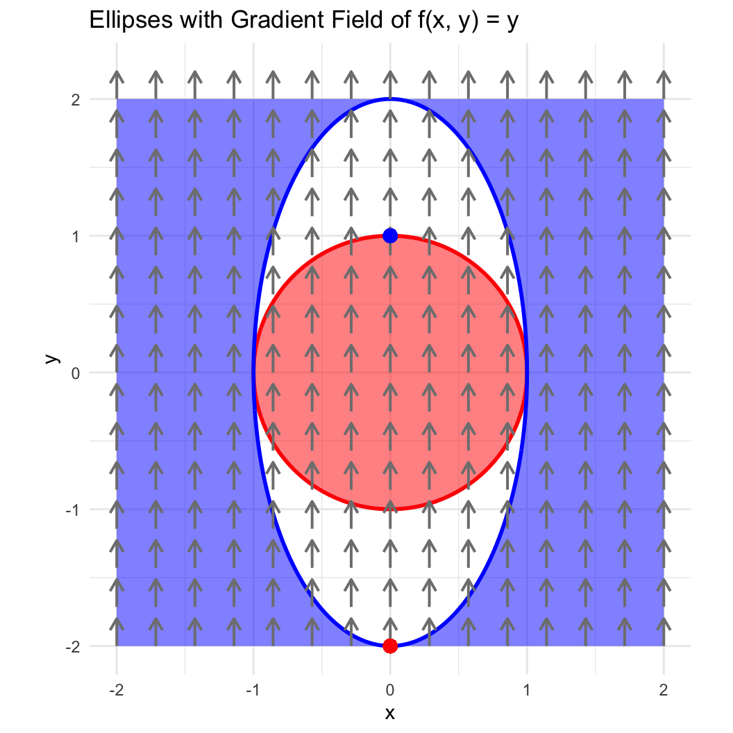
The white area is the feasible region of the problem. The red point is the constrained minimum.

Lagrangian Function

We define the Lagrangian function as follows:

\mathcal{L}(x,y,\mu_1,\mu_2) = y - \mu_1(x^2 + y^2 - 1) - \mu_2\left(1 - x^2 - \frac{1}{4}y^2\right)

First-Order Conditions

The first-order conditions derived from the Lagrangian are:

\begin{aligned} \frac{\partial \mathcal{L}}{\partial x} &= 2x(\mu_2 - \mu_1), \\ \frac{\partial \mathcal{L}}{\partial y} &= 1 + y\left(\frac{1}{2}\mu_2 - 2\mu_1\right), \\ 0 &= \mu_1(x^2 + y^2 - 1), \\ 0 &= \mu_2\left(1 - x^2 - \frac{1}{4}y^2\right). \end{aligned}

Solutions of First-Order Conditions

The solutions to the first-order conditions yield the following critical points:

\begin{aligned} x &= 0, & y &= 1, & \mu_1 &= \frac{1}{2}, & \mu_2 &= 0, \\ x &= 0, & y &= -2, & \mu_1 &= 0, & \mu_2 &= 1. \end{aligned}

Analysis of First Candidate

Compute Active Constraints

We evaluate the constraints at the first candidate (x, y) = (0, 1):

\begin{aligned} g_1(x,y) &= x^2 + y^2 - 1 = 0^2 + 1^2 - 1 = 0, & \text{(active)} \\ g_2(x,y) &= 1 - x^2 - \frac{1}{4}y^2 = 1 - 0^2 - \frac{1}{4}1^2 = \frac{3}{4} > 0, & \text{(not-active)} \end{aligned}

Gradient of Active Constraints

The gradient of the active constraint g_1 is computed as follows:

\nabla g_1(x,y) = [2x, 2y] = [0, 2].

Check qualification

The single active gradient \nabla g_1(x,y)=[0,2] is nonzero, so LICQ holds.

Kernel of the Gradient of Active Constraints

The kernel of the gradient can be expressed as:

[0, 2] \begin{pmatrix} z_1 \\ z_2 \end{pmatrix} = 2z_2 = 0 \implies \begin{pmatrix} z_1 \\ z_2 \end{pmatrix} = \begin{pmatrix} \alpha \\ 0 \end{pmatrix} = \underbrace{\begin{pmatrix} 1 \\ 0 \end{pmatrix}}_{\bm{K}^a} \alpha.

Reduced Hessian

The reduced Hessian is given by:

\begin{aligned} \nabla^2_{(x,y)} \mathcal{L}(x,y,\mu_1,\mu_2) &= \begin{pmatrix} 2(\mu_2 - \mu_1) & 0 \\ 0 & \frac{1}{2}(\mu_2 - 4\mu_1) \end{pmatrix} \\ & \implies \begin{pmatrix} -1 & 0 \\ 0 & -1 \end{pmatrix}. \end{aligned}

Evaluating the quadratic form yields:

\begin{aligned} \bm{K}^{a,\top} \nabla^2_{(x,y)} \mathcal{L}(x,y,\mu_1,\mu_2) \bm{K}^a &= \begin{pmatrix} 1 & 0 \end{pmatrix} \begin{pmatrix} -1 & 0 \\ 0 & -1 \end{pmatrix} \begin{pmatrix} 1 \\ 0 \end{pmatrix} = -1. \end{aligned}

Because \mu_1=1/2>0, the critical cone is the tangent line z_2=0. The reduced Hessian equals -1 on that line, so the second-order necessary condition fails and this point is not a local minimum.

---

Analysis of Second Candidate

Compute Active Constraints

Next, we evaluate the constraints at the second candidate (x, y) = (0, -2):

\begin{aligned} g_1(x,y) &= x^2 + y^2 - 1 = 0^2 + (-2)^2 - 1 = 3 > 0, & \text{(not-active)} \\ g_2(x,y) &= 1 - x^2 - \frac{1}{4}y^2 = 1 - 0^2 - \frac{1}{4}(-2)^2 = 0, & \text{(active)} \end{aligned}

Gradient of Active Constraints

The gradient of the active constraint g_2 is computed as:

\nabla g_2(x,y) = [-2x, -\tfrac{1}{2}y] = [0, 1].

Check qualification

The single active gradient \nabla g_2(x,y)=[0,1] is nonzero, so LICQ holds.

Kernel of the Gradient of Active Constraints

The kernel of the gradient can be expressed as:

[0, 1] \begin{pmatrix} z_1 \\ z_2 \end{pmatrix} = z_2 = 0 \implies \begin{pmatrix} z_1 \\ z_2 \end{pmatrix} = \begin{pmatrix} \alpha \\ 0 \end{pmatrix} = \underbrace{\begin{pmatrix} 1 \\ 0 \end{pmatrix}}_{\bm{K}^a} \alpha.

Reduced Hessian

The reduced Hessian is given by:

\begin{aligned} \nabla^2_{(x,y)} \mathcal{L}(x,y,\mu_1,\mu_2) &= \begin{pmatrix} 2(\mu_2 - \mu_1) & 0 \\ 0 & \frac{1}{2}(\mu_2 - 4\mu_1) \end{pmatrix} \\ & \implies \begin{pmatrix} 2 & 0 \\ 0 & \frac{1}{2} \end{pmatrix}. \end{aligned}

Evaluating the quadratic form yields:

\begin{aligned} \bm{K}^{a,\top} \nabla^2_{(x,y)} \mathcal{L}(x,y,\mu_1,\mu_2) \bm{K}^a &= \begin{pmatrix} 1 & 0 \end{pmatrix} \begin{pmatrix} 2 & 0 \\ 0 & \frac{1}{2} \end{pmatrix} \begin{pmatrix} 1 \\ 0 \end{pmatrix} = 2. \end{aligned}

Because the active multiplier is \mu_2=1>0, the critical cone equals this tangent line. The reduced Hessian is positive definite on it, so the second-order sufficient condition holds and (0,-2) is a strict local minimum.

Example 4

Consider the problem

\begin{aligned} \text{minimize:}\quad & f(x, y) = x \\ \text{inequalities:}\quad & g_1(x,y) = x^2+y^2-1 \geq 0, \\ & g_2(x,y) = 1-x^2-\frac{1}{4}y^2 \geq 0, \end{aligned}

Figure 1.3: Feasible region and constrained minimum for the alternative objective.

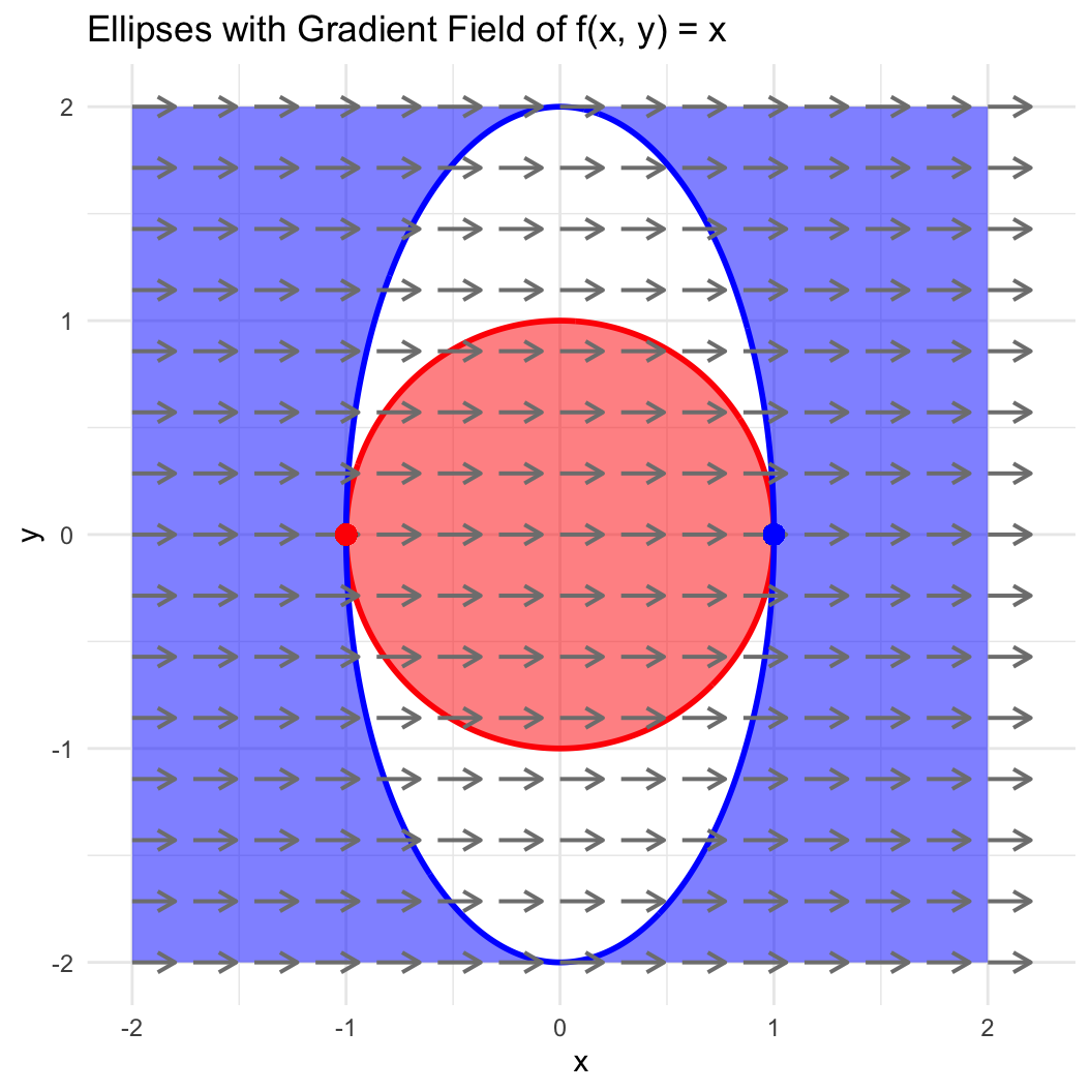
The white area is the feasible region of the problem. The red point is the constrained minimum.

Lagrangian Function

We define the Lagrangian function as follows:

\mathcal{L}(x,y,\mu_1,\mu_2) = x - \mu_1(x^2 + y^2 - 1) - \mu_2\left(1 - x^2 - \frac{1}{4}y^2\right)

First-Order Conditions

The first-order conditions derived from the Lagrangian are:

\begin{aligned} \frac{\partial \mathcal{L}}{\partial x} &= 1+2x(\mu_2 - \mu_1), \\ \frac{\partial \mathcal{L}}{\partial y} &= y\left(\frac{1}{2}\mu_2 - 2\mu_1\right), \\ 0 &= \mu_1(x^2 + y^2 - 1), \\ 0 &= \mu_2\left(1 - x^2 - \frac{1}{4}y^2\right). \end{aligned}

Solutions of First-Order Conditions

• Case y=0 \begin{aligned} 0 &= 1+2x(\mu_2 - \mu_1), \\ 0 &= \mu_1(x^2 - 1), \\ 0 &= \mu_2(1 - x^2). \end{aligned}

  in this case if \mu_1=\mu_2=0 the first equation fails. Thus x=1 or x=-1

  • Case x=1 solving 1+2(\mu_2 - \mu_1)=0 we have \mu_1=1/2+\mu_2
  • Case x=-1 solving 1-2(\mu_2 - \mu_1)=0 we have \mu_2=1/2+\mu_1

  thus we have two family of solution

  • x=1, y=0, \mu_1=1/2+\mu_2 with \mu_1\geq 0
  • x=-1, y=0, \mu_2=1/2+\mu_1 with \mu_2\geq 0

• Case y\neq 0 in this case \mu_2=4\mu_1 and \left\{ \begin{aligned} 0 &= 1+6x\mu_1, \\ 0 &= \mu_1(x^2 + y^2 - 1), \\ 0 &= 4\mu_1\left(1 - x^2 - \frac{1}{4}y^2\right). \end{aligned}\right. \implies \mu_1\neq 0\implies \left\{ \begin{aligned} 0 &= x^2 + y^2 - 1, \\ 0 &= 1 - x^2 - \frac{1}{4}y^2. \end{aligned}\right. but the last system has solution y=0 and x=\pm1. Thus the solution must be discarded.

The solutions to the first-order conditions yield the following critical points:

\begin{aligned} x &= 1, & y &= 0, & \mu_1 &= \frac{1}{2}+\mu_2, \\ x &= -1, & y &= 0, & \mu_2 &= \frac{1}{2}+\mu_1 \end{aligned}

Analysis of the candidate (1,0)

Both inequalities are active: g_1(1,0)=g_2(1,0)=0. Their gradients are \nabla g_1(1,0)=(2,0)^\top, \qquad \nabla g_2(1,0)=(-2,0)^\top. Thus LICQ fails. In fact MFCQ fails as well: there is no direction d such that simultaneously \nabla g_1(1,0)^\top d>0, \qquad \nabla g_2(1,0)^\top d>0, because these two inequalities require d_1>0 and d_1<0 at the same time. The KKT multipliers are therefore nonunique: \mu_1=\frac12+\mu_2, \qquad \mu_2\ge0.

Because the standard constraint qualifications fail, it is safer not to infer minimality from a reduced-Hessian test alone. A direct feasible curve settles the question. For small t define x(t)=\sqrt{1-t^2}, \qquad y(t)=t. Then g_1(x(t),y(t))=0 and g_2(x(t),y(t)) =1-(1-t^2)-\frac14t^2 =\frac34t^2\ge0, so the curve is feasible. Moreover, f(x(t),y(t))=x(t)=\sqrt{1-t^2}<1=f(1,0) \qquad(t\ne0). Hence (1,0) is not a local minimum (indeed it is the local maximum of x on the feasible lens near that point).

Analysis of the candidate (-1,0)

Again both inequalities are active and \nabla g_1(-1,0)=(-2,0)^\top, \qquad \nabla g_2(-1,0)=(2,0)^\top, so LICQ and MFCQ fail. The KKT multipliers are nonunique: \mu_2=\frac12+\mu_1, \qquad \mu_1\ge0.

Nevertheless, minimality is immediate from the second inequality alone. Every feasible point satisfies x^2+\frac14y^2\le1, and therefore x\ge-1. Equality x=-1 forces y=0. Consequently f(x,y)=x\ge-1=f(-1,0) for every feasible point, with equality only at (-1,0). Thus (-1,0) is in fact the unique global minimum.

This example is useful precisely because the usual LICQ-based second-order KKT test is not applicable at the two intersection points. The geometry of the feasible set (or a more general second-order theory for degenerate constraints) must be used instead.

Example 5

Consider the problem

\begin{aligned} \text{minimize:}\quad & f(x,y) = 6 + 2y-x^2 \\ \text{equality:}\quad & h(x,y) = y - x^2 \end{aligned}

Lagrangian function

\mathcal{L}(x,y,\lambda) = 6 + 2y-x^2 - \lambda(y - x^2)

First-Order Conditions

\begin{aligned} \frac{\partial\mathcal{L}}{\partial x} & = 2x(\lambda-1) = 0\\ \frac{\partial\mathcal{L}}{\partial y} & = 2 - \lambda = 0\\ 0 & = y - x^2 \end{aligned}

Solution First-Order Conditions

• \lambda = 2
• x=0
• y=0

Analysis of the Candidate

Gradient of the constraints

\nabla (y - x^2) = \begin{pmatrix} -2x & 1 \end{pmatrix},\quad \implies\quad \begin{pmatrix} 0 & 1 \end{pmatrix}

Check Qualification

The gradient (0,1) is nonzero, hence LICQ holds.

Kernel of the Gradient of Active Constraints

\begin{pmatrix} 0 & 1 \end{pmatrix} \begin{pmatrix} z_1 \\ z_2 \end{pmatrix} = z_2 = 0,\quad \implies\quad \begin{pmatrix} z_1 \\ z_2 \end{pmatrix} = \begin{pmatrix} \alpha \\ 0 \end{pmatrix} = \underbrace{\begin{pmatrix} 1 \\ 0 \end{pmatrix}}_{\bm{K}^a} \alpha

Reduced Hessian

\nabla^2_{(x,y)}\mathcal{L}(x,y,\lambda) = \begin{pmatrix} 2(\lambda - 1) & 0 \\ 0 & 0 \end{pmatrix} \quad\implies\quad \begin{pmatrix} 2 & 0 \\ 0 & 0 \end{pmatrix}

\bm{K}^{a,\top} \nabla^2_{(x,y)}\mathcal{L}(0,0,2) \bm{K}^{a} = \begin{pmatrix} 1 & 0 \end{pmatrix} \begin{pmatrix} 2 & 0 \\ 0 & 0 \end{pmatrix} \begin{pmatrix} 1 \\ 0 \end{pmatrix} = (2)

The reduced Hessian is positive definite. Therefore the second-order sufficient condition holds and (0,0) is a strict local minimum. In fact, substituting y=x^2 into the objective gives f=6+x^2, so this minimum is global.

Why the curvature of the constraint matters

A useful companion test compares two constraints having exactly the same tangent space at the candidate. Consider

f(x,y)=3+y-\frac12x^2

with either

h_c(x,y)=y-x^2=0 \qquad\text{or}\qquad h_s(x,y)=y=0.

At (0,0),

\nabla h_c(0,0)=\nabla h_s(0,0)=(0,1)^\top,

so the two feasible curves have the same tangent line. The first-order Lagrange conditions also give the same multiplier, \lambda=-1, if the convention \mathcal L=f+\lambda h is used. Nevertheless,

\nabla^2 f(0,0)= \begin{pmatrix}-1&0\\0&0\end{pmatrix},

while

\nabla^2_{(x,y)}\mathcal L_c(0,0,-1) = \begin{pmatrix}1&0\\0&0\end{pmatrix}, \qquad \nabla^2_{(x,y)}\mathcal L_s(0,0,-1) = \begin{pmatrix}-1&0\\0&0\end{pmatrix}.

The common tangent space is spanned by \bm z=(1,0)^\top. Hence

\bm z^\top\nabla^2\mathcal L_c\bm z=1>0, \qquad \bm z^\top\nabla^2\mathcal L_s\bm z=-1<0.

Thus (0,0) is a strict local minimum on the parabola y=x^2, but a strict local maximum on the line y=0. This small example is important: for curved constraints, the correct second-order object is the Hessian of the Lagrangian, not the Hessian of the objective alone. This is the standard second-order KKT principle; see Nocedal and Wright, Numerical Optimization, 2nd ed., Section 12.4.

1.3 Example 6: A Three-Variable KKT Test with a Weakly Active Constraint

Consider

\begin{aligned} \min_{x,y,z}\quad & f(x,y,z)=-x^3+y^2-2xz^2,\\ \text{subject to}\quad & h(x,y,z)=2x+y^2+z-5=0,\\ & g_1(x,y,z)=5x^2-y^2-z-2\ge0,\\ & g_2(x,y,z)=x\ge0,\qquad g_3(x,y,z)=y\ge0,\qquad g_4(x,y,z)=z\ge0. \end{aligned}

Using the convention

\mathcal L=f-\lambda h-\sum_{j=1}^4\mu_j g_j, \qquad \mu_j\ge0,

the KKT equations admit

\bm x^\star=(1,0,3)^\top, \qquad \lambda^\star=-\frac{47}{4}, \qquad \mu_1^\star=\frac14, \qquad \mu_2^\star=\mu_3^\star=\mu_4^\star=0.

At this point h, g_1, and g_3 are active. Their gradients are

\nabla h=(2,0,1)^\top, \qquad \nabla g_1=(10,0,-1)^\top, \qquad \nabla g_3=(0,1,0)^\top.

They are linearly independent, so LICQ holds.

The critical cone, not merely the null space of all active gradients

There is a subtle point in this exercise. Since \mu_3^\star=0, the active constraint y\ge0 is weakly active. For second-order conditions we should therefore use the critical cone. The equalities associated with h and with the strictly positive multiplier \mu_1^\star give

2d_x+d_z=0, \qquad 10d_x-d_z=0,

hence d_x=d_z=0. The weakly active bound gives d_y\ge0. Thus

\mathcal C(\bm x^\star,\bm\mu^\star) = \{(0,\eta,0)^\top:\eta\ge0\}.

The Hessian of the Lagrangian at the KKT point is

\nabla^2_{\bm x\bm x}\mathcal L(\bm x^\star,\lambda^\star,\bm\mu^\star) = \begin{pmatrix} -\frac{17}{2} & 0 & -12\\ 0 & 26 & 0\\ -12 & 0 & -4 \end{pmatrix}.

For every nonzero critical direction \bm d=(0,\eta,0)^\top,

\bm d^\top\nabla^2\mathcal L\bm d=26\eta^2>0.

Hence the second-order sufficient condition holds and \bm x^\star is a strict local minimizer. This example is particularly useful for distinguishing active constraints from strongly active constraints and for motivating the critical cone used in the general second-order KKT theory.

1.4 Example 7: Chong–Zak Maximum-Power-Transfer Test

This is a standard textbook example; it appears as Example 20.2 in Chong and Zak, An Introduction to Optimization. A 20 V source feeds two series resistors, a fixed 10\,\Omega resistor and a variable resistor R\ge0. Let i be the circuit current. The power absorbed by R is P=Ri^2, so the maximization can be written as

\begin{aligned} \min_{R,i}\quad & -Ri^2,\\ \text{subject to}\quad &20-(R+10)i=0,\\ &R\ge0. \end{aligned}

With

\mathcal L=-Ri^2-\lambda[20-(R+10)i]-\mu R,

the interior KKT solution is

R^\star=10, \qquad i^\star=1, \qquad \lambda^\star=1, \qquad \mu^\star=0.

The bound is inactive. The equality-gradient row is

\nabla h(R^\star,i^\star)=(-1,-20),

so a tangent direction is \bm z=(-20,1)^\top. Moreover,

\nabla^2_{(R,i)}\mathcal L(R^\star,i^\star) = \begin{pmatrix}0&-1\\-1&-20\end{pmatrix},

and

\bm z^\top\nabla^2\mathcal L\bm z=20>0.

Thus the point is a strict local minimum of -Ri^2, equivalently a strict local maximum of the absorbed power. Eliminating the equality gives

P(R)=\frac{400R}{(R+10)^2},

whose unique maximizer on R\ge0 is R=10\,\Omega. This is the familiar maximum power transfer theorem for a purely resistive source/load network.

1.5 Example 8: Maximum-Volume Rectangular Box with Fixed Surface Area

A classical geometric optimization problem is to maximize the volume of a rectangular box with fixed surface area. With the normalization used here,

\begin{aligned} \min_{x,y,z}\quad & -xyz,\\ \text{subject to}\quad &2(xy+yz+xz)-1=0,\\ &x\ge0,\qquad y\ge0,\qquad z\ge0. \end{aligned}

At an interior solution the bound multipliers vanish. By symmetry, or directly from the KKT equations,

x^\star=y^\star=z^\star=\frac1{\sqrt6}, \qquad \lambda^\star=-\frac{\sqrt6}{24}.

(The all-negative stationary point of the equality-constrained equations is not feasible and must be discarded once the nonnegativity constraints are included.)

A basis for the tangent space of the equality constraint is, for example,

\bm Z= \begin{pmatrix} -1&-1\\ 0&1\\ 1&0 \end{pmatrix}.

The reduced Hessian is

\bm Z^\top\nabla^2\mathcal L(\bm x^\star,\lambda^\star)\bm Z = \begin{pmatrix} \frac{\sqrt6}{6} & \frac{\sqrt6}{12}\\ \frac{\sqrt6}{12} & \frac{\sqrt6}{6} \end{pmatrix},

whose leading principal minors are positive. Hence the second-order sufficient condition holds.

There is also a short global argument. Since

xy+yz+xz=\frac12,

AM–GM gives

\frac{xy+yz+xz}{3} \ge \sqrt[3]{(xy)(yz)(xz)} =(xyz)^{2/3},

and therefore

xyz\le\frac{1}{6\sqrt6},

with equality only for xy=yz=xz, hence x=y=z=1/\sqrt6. Thus the KKT candidate is the unique global maximizer of the volume.

1.6 Example 9: Nonconvex Objective on an Elliptic Feasible Set

Consider the course test

\begin{aligned} \min_{x,y}\quad &f(x,y)=x^2\left(1+\frac1{10}\sin(1-10x)\right)+y^2-e^y,\\ \text{subject to}\quad &g(x,y)=1-x^2-2y^2\ge0. \end{aligned}

The feasible set is the ellipse x^2+2y^2\le1. Numerical solution of the KKT system gives the boundary candidate

x^\star=0, \qquad y^\star=\frac1{\sqrt2}, \qquad \mu^\star\approx0.2170469283.

For the convention \mathcal L=f-\mu g, the tangent space to the active constraint is spanned by \bm z=(1,0)^\top. The important detail is that the second-order test must use the Hessian of the Lagrangian:

\nabla^2\mathcal L = \nabla^2 f-\mu\nabla^2g.

At the candidate,

\bm z^\top\nabla^2\mathcal L\bm z = f_{xx}(0,1/\sqrt2)+2\mu^\star \approx 2.6024>0.

Thus the second-order sufficient condition is satisfied on the one-dimensional critical/tangent space, and the candidate is a strict local minimizer. This example is not a widely standardized named benchmark; it is useful as a compact numerical KKT test with a nonconvex objective and an active curved inequality.

1.7 Example 10: A Linear Objective on the Unit Sphere

Consider

\begin{aligned} \min_{\bm x\in\mathbb R^3}\quad & f(\bm x)=x+y+z,\\ \text{subject to}\quad & h(\bm x)=x^2+y^2+z^2-1=0. \end{aligned}

This is a useful first equality-constrained problem because the geometry is completely transparent and the same answer can be obtained by parameterization, by Cauchy–Schwarz, or by Lagrange multipliers. The original exercise develops both a spherical parameterization and the multiplier approach; here we emphasize the latter and use the parameterization only as a geometric check.

The Lagrangian is

\mathcal L(\bm x,\lambda) =x+y+z-\lambda(x^2+y^2+z^2-1).

The first-order conditions are

\nabla_{\bm x}\mathcal L = \begin{bmatrix}1\\1\\1\end{bmatrix} -2\lambda \begin{bmatrix}x\\y\\z\end{bmatrix} =\bm0, \qquad x^2+y^2+z^2=1.

Hence

x=y=z=\frac{1}{2\lambda},

and therefore

3\frac{1}{4\lambda^2}=1, \qquad \lambda=\pm\frac{\sqrt3}{2}.

The two stationary points are

\bm x_+=\frac1{\sqrt3}\begin{bmatrix}1\\1\\1\end{bmatrix}, \qquad \bm x_-=-\frac1{\sqrt3}\begin{bmatrix}1\\1\\1\end{bmatrix}.

Their objective values are

f(\bm x_+)=\sqrt3, \qquad f(\bm x_-)=-\sqrt3.

Thus \bm x_- is the global minimum and \bm x_+ is the global maximum. This also follows immediately from Cauchy–Schwarz:

|x+y+z| \le \sqrt{1^2+1^2+1^2}\sqrt{x^2+y^2+z^2} =\sqrt3.

At either point the tangent space is

T(\bm x_\pm) = \left\{\bm d:\bm x_\pm^{\mathsf T}\bm d=0\right\}.

Since

\nabla^2_{\bm x\bm x}\mathcal L=-2\lambda\bm I,

the reduced Hessian is positive definite at \bm x_- and negative definite at \bm x_+.

The main lesson is that the multiplier condition is simply the normality condition

\nabla f(\bm x^\star)\in\operatorname{span}\{\nabla h(\bm x^\star)\}.

1.8 Example 11: Two Equality Constraints in \mathbb R^3

Consider

\begin{aligned} \min_{x,y,z}\quad & f(x,y,z)=x^2-z,\\ \text{subject to}\quad & h_1(x,y,z)=y-x^2=0,\\ & h_2(x,y,z)=x+y+z-1=0. \end{aligned}

This problem is especially useful because it can first be reduced to one variable by eliminating the constraints, and then solved again with Lagrange multipliers and a reduced Hessian.

Direct elimination

From the constraints,

y=x^2, \qquad z=1-x-x^2.

Therefore

\widehat f(x) =x^2-(1-x-x^2) =2x^2+x-1.

Hence

\widehat f'(x)=4x+1=0, \qquad x^\star=-\frac14,

and

\widehat f''(x)=4>0.

Thus

\boxed{ \bm x^\star= \begin{bmatrix} -1/4\\[2pt]1/16\\[2pt]19/16 \end{bmatrix}}

is a strict minimum along the feasible curve.

Lagrange multiplier calculation

Using

\mathcal L =f-\lambda_1 h_1-\lambda_2 h_2,

stationarity gives

\begin{aligned} 2x+2\lambda_1x-\lambda_2&=0,\\ -\lambda_1-\lambda_2&=0,\\ -1-\lambda_2&=0. \end{aligned}

Therefore

\lambda_2=-1, \qquad \lambda_1=1, \qquad x=-\frac14,

which reproduces the point obtained by elimination.

The constraint Jacobian at \bm x^\star is

\bm J_h(\bm x^\star) = \begin{bmatrix} 1/2 & 1 & 0\\ 1 & 1 & 1 \end{bmatrix}.

It has rank two, so LICQ holds. A basis of the one-dimensional tangent space is

\bm Z= \begin{bmatrix}2\\-1\\-1\end{bmatrix}, \qquad \bm J_h\bm Z=\bm0.

With the sign convention above,

\nabla^2_{\bm x\bm x}\mathcal L(\bm x^\star) = \begin{bmatrix} 4&0&0\\ 0&0&0\\ 0&0&0 \end{bmatrix},

and the reduced Hessian is the scalar

\bm Z^{\mathsf T} \nabla^2_{\bm x\bm x}\mathcal L \bm Z =16>0.

Therefore the second-order sufficient condition is satisfied.

This example makes the dimension count explicit:

\dim T=n-m=3-2=1.

1.9 Example 12: Positive Curvature Only on the Constraint Kernel

Second-order constrained optimality does not require the Hessian to be positive definite in the entire ambient space. It only needs positive curvature along feasible first-order directions.

The historical worksheet motivating this example uses

\bm A= \begin{bmatrix} 4&1&1&-4\\ 1&2&1&1\\ 1&1&4&-1\\ -4&-1&1&2 \end{bmatrix}, \qquad \bm B= \begin{bmatrix} 1&1&1&2\\ 1&1&0&1 \end{bmatrix}.

There is an important technical point: the displayed \bm A is not symmetric, so it is not meaningful to call \bm A itself SPD. For a quadratic form only the symmetric part matters. Define

\bm S=\frac12(\bm A+\bm A^{\mathsf T}) = \begin{bmatrix} 4&1&1&-4\\ 1&2&1&0\\ 1&1&4&0\\ -4&0&0&2 \end{bmatrix}.

The kernel of \bm B can be written as

\bm d= \begin{bmatrix} -y+z\\y\\z\\-z \end{bmatrix} = \bm Z \begin{bmatrix}z\\y\end{bmatrix}, \qquad \bm Z= \begin{bmatrix} 1&-1\\ 0&1\\ 1&0\\ -1&0 \end{bmatrix}.

The symmetric reduced matrix is

\bm Z^{\mathsf T}\bm S\bm Z = \begin{bmatrix} 20&-7\\ -7&4 \end{bmatrix}.

By Sylvester’s criterion,

20>0, \qquad \det\begin{bmatrix}20&-7\\-7&4\end{bmatrix}=31>0,

hence

\bm Z^{\mathsf T}\bm S\bm Z\succ0.

Equivalently, for every nonzero \bm d\in\ker\bm B,

\bm d^{\mathsf T}\bm S\bm d =4y^2-14yz+20z^2>0.

Thus the quadratic form has positive curvature on the feasible tangent subspace even though positivity in the full ambient space is not required.

This is the algebraic core of the reduced-Hessian test used throughout the KKT examples.

1.10 Example 13: Box Constraints, Active Sets, and KKT Filtering

Consider the box-constrained problem

\begin{aligned} \min_{x,y}\quad & f(x,y)=y-x^2+x,\\ \text{subject to}\quad & -1\le x\le1,\\ & -1\le y\le1. \end{aligned}

Write the inequalities in the course convention g_i\ge0:

\begin{aligned} g_1&=1-x, & g_2&=x+1,\\ g_3&=1-y, & g_4&=y+1. \end{aligned}

The Lagrangian is

\mathcal L =f-\sum_{i=1}^4\mu_i g_i, \qquad \mu_i\ge0.

Stationarity gives

\begin{aligned} 1-2x+\mu_1-\mu_2&=0,\\ 1+\mu_3-\mu_4&=0, \end{aligned}

together with

\mu_i g_i=0, \qquad g_i\ge0, \qquad \mu_i\ge0.

There is no unconstrained stationary point because

\frac{\partial f}{\partial y}=1.

Consequently every constrained minimizer must lie on the boundary. The KKT system produces three feasible dual-feasible candidates.

Candidate A: (-1,-1)

The active constraints are g_2=g_4=0. Stationarity yields

\mu_2=3, \qquad \mu_4=1,

with the remaining multipliers zero. Since both active multipliers are strictly positive, the critical cone is reduced to \{\bm0\} at this corner. Direct evaluation confirms

f(-1,-1)=-3.

Candidate B: (1,-1)

Here g_1=g_4=0 and

\mu_1=1, \qquad \mu_4=1.

Again the critical cone at the vertex is trivial. The objective value is

f(1,-1)=-1.

This point is a local minimum at the corner, but not the global one.

Candidate C: (1/2,-1)

Only g_4 is active, with

\mu_4=1.

The feasible tangent direction is horizontal,

\bm d=\begin{bmatrix}d_x\\0\end{bmatrix}.

Since

\nabla^2 f = \begin{bmatrix}-2&0\\0&0\end{bmatrix},

we obtain

\bm d^{\mathsf T}\nabla^2 f\,\bm d =-2d_x^2<0 \qquad(d_x\ne0).

Thus this KKT point is not a local minimum; it is a saddle point relative to the box.

The remaining boundary stationary points that appear if one enumerates faces without enforcing multiplier signs are rejected by dual feasibility. In particular, the maximizer

\left(\frac12,1\right)

is not a KKT point for the minimization problem with the sign convention g_i\ge0, \mathcal L=f-\sum_i\mu_i g_i, \mu_i\ge0.

Finally, because f is increasing in y, the global minimizer must have y=-1. On that edge,

f(x,-1)=-1-x^2+x,

which is concave, so its minimum over [-1,1] occurs at an endpoint. Comparing -3 and -1 gives

\boxed{(x^\star,y^\star)=(-1,-1)}, \qquad \boxed{f^\star=-3}.

1.11 Example 14: A Mixed Equality–Inequality Problem with a Strict Local Minimum

Consider

\min_{x,y,z}\; f(x,y,z)=-xyz-z

subject to

h(x,y,z)=x+y-1=0, \qquad g(x,y,z)=2-z\ge 0.

This example is useful because it contains both an equality and an inequality constraint, it has several KKT points, and the strict local minimizer is not a global minimizer.

With the convention g\ge0, define

\mathcal L(x,y,z,\lambda,\mu) = -xyz-z-\lambda(x+y-1)-\mu(2-z), \qquad \mu\ge0.

The KKT conditions are

\begin{aligned} -yz-\lambda &=0,\\ -xz-\lambda &=0,\\ -xy-1+\mu &=0,\\ x+y-1&=0,\\ \mu(2-z)&=0,\\ \mu&\ge0, \qquad 2-z\ge0. \end{aligned}

Subtracting the first two stationarity equations gives

z(x-y)=0.

Active inequality: z=2

If \mu>0, complementarity gives z=2. Then the first two stationarity equations imply x=y, and the equality constraint gives

x^\star=y^\star=\frac12, \qquad z^\star=2.

The multipliers are

\lambda^\star=-1, \qquad \mu^\star=1+x^\star y^\star=\frac54>0.

Hence

\bm x^\star= \begin{bmatrix} 1/2\\[1mm]1/2\\[1mm]2 \end{bmatrix}

satisfies the KKT conditions with the inequality strongly active.

The gradients of the active constraints are

\nabla h(\bm x^\star)= \begin{bmatrix}1\\1\\0\end{bmatrix}, \qquad \nabla g(\bm x^\star)= \begin{bmatrix}0\\0\\-1\end{bmatrix},

which are linearly independent. Therefore LICQ holds. The tangent space to the active constraints is

\mathcal T = \left\{\bm d:\; d_x+d_y=0,\ d_z=0\right\} = \operatorname{span} \left\{ \begin{bmatrix}1\\-1\\0\end{bmatrix} \right\}.

Since both constraints are affine, the Hessian of the Lagrangian is just the Hessian of the objective,

\nabla^2_{\bm x\bm x}\mathcal L = \begin{bmatrix} 0 & -z & -y\\ -z & 0 & -x\\ -y & -x & 0 \end{bmatrix}.

At \bm x^\star,

\bm H^\star= \begin{bmatrix} 0 & -2 & -1/2\\ -2 & 0 & -1/2\\ -1/2 & -1/2 & 0 \end{bmatrix}.

For \bm d=\alpha(1,-1,0)^T,

\bm d^T\bm H^\star\bm d=4\alpha^2>0 \qquad (\alpha\ne0).

Therefore \bm x^\star is a strict local minimizer.

Inactive inequality: two additional KKT points

If \mu=0, stationarity in z gives xy=-1. Together with x+y=1,

x=\frac{1\pm\sqrt5}{2}, \qquad y=\frac{1\mp\sqrt5}{2}.

The first two stationarity equations then force z=0 and \lambda=0. Thus there are two additional KKT points,

\left( \frac{1\pm\sqrt5}{2}, \frac{1\mp\sqrt5}{2}, 0 \right),

but they are saddle points. Indeed, after eliminating y=1-x the objective becomes

\phi(x,z)=-z\left(1+x-x^2\right),

and at either of the above points its Hessian has eigenvalues of opposite sign.

Finally, the problem is not globally bounded below. For instance, with z=-1 and y=1-x,

f(x,1-x,-1)=1+x-x^2\longrightarrow-\infty \qquad\text{as }|x|\to\infty.

Thus this example also illustrates the distinction between a strict local minimizer and a global minimizer.

{#fig-kkt-mixed-local-minimum fig-align=“center” width=“85%”,bg=“white”}

1.12 Example 15: KKT Filtering with an Elliptic Constraint and Box Constraint in z

Consider

\min_{x,y,z}\; f(x,y,z)=x+y^2-z

subject to

g_1(x,y,z)=1-\frac{x^2}{2}-y^2\ge0, \qquad g_2(x,y,z)=z\ge0, \qquad g_3(x,y,z)=1-z\ge0.

The feasible set is an elliptic cylinder truncated by the planes z=0 and z=1.

The Lagrangian is

\mathcal L =x+y^2-z -\mu_1\left(1-\frac{x^2}{2}-y^2\right) -\mu_2 z -\mu_3(1-z),

with \mu_i\ge0. Stationarity gives

\begin{aligned} 1+\mu_1x&=0,\\ 2y(1+\mu_1)&=0,\\ -1-\mu_2+\mu_3&=0. \end{aligned}

Together with

\mu_1g_1=0, \qquad \mu_2z=0, \qquad \mu_3(1-z)=0,

these equations allow a short active-set analysis.

Because 1+\mu_1x=0, we must have \mu_1>0. Hence g_1=0. Since \mu_1\ge0,

2y(1+\mu_1)=0 \quad\Longrightarrow\quad y=0.

Thus

1-\frac{x^2}{2}=0,

and stationarity in x selects the negative root,

x^\star=-\sqrt2, \qquad \mu_1^\star=\frac{1}{\sqrt2}.

For the z constraints, an interior value 0<z<1 would imply \mu_2=\mu_3=0, contradicting the third stationarity equation. At z=0, one would obtain \mu_2=-1, which violates dual feasibility. Therefore

z^\star=1, \qquad \mu_2^\star=0, \qquad \mu_3^\star=1.

The unique KKT point is therefore

\boxed{ \bm x^\star=(-\sqrt2,0,1)^T }

with

\boxed{ \bm\mu^\star= \left(\frac1{\sqrt2},0,1\right)^T. }

The active constraints are g_1 and g_3. Their gradients are

\nabla g_1(\bm x^\star)= \begin{bmatrix}\sqrt2\\0\\0\end{bmatrix}, \qquad \nabla g_3(\bm x^\star)= \begin{bmatrix}0\\0\\-1\end{bmatrix},

so LICQ holds and

\mathcal T = \operatorname{span} \left\{ \begin{bmatrix}0\\1\\0\end{bmatrix} \right\}.

The Hessian of the Lagrangian is

\nabla^2_{\bm x\bm x}\mathcal L = \begin{bmatrix} \mu_1 & 0 & 0\\ 0 & 2+2\mu_1 & 0\\ 0 & 0 & 0 \end{bmatrix}.

At the KKT point, for \bm d=\alpha(0,1,0)^T,

\bm d^T\nabla^2_{\bm x\bm x}\mathcal L(\bm x^\star,\bm\mu^\star)\bm d =(2+\sqrt2)\alpha^2>0 \qquad(\alpha\ne0).

Hence the second-order sufficient condition holds and \bm x^\star is a strict local minimizer.

In this case one can also prove global optimality directly. Since -z is minimized by z=1, it remains to minimize

x+y^2

over x^2/2+y^2\le1. For fixed y the smallest admissible x is

x=-\sqrt{2(1-y^2)},

so the reduced problem is

\min_{|y|\le1} \left[-\sqrt{2(1-y^2)}+y^2\right],

whose unique minimizer is y=0. Therefore \bm x^\star is the unique global minimizer.

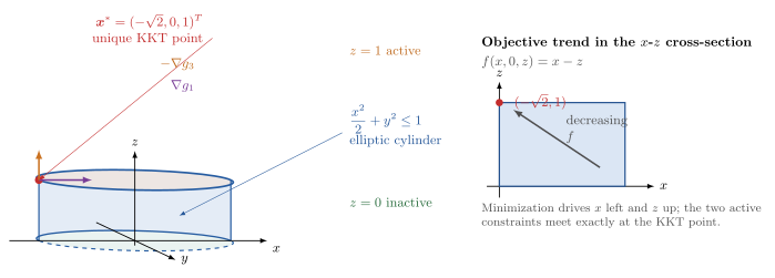{#fig-kkt-elliptic-cylinder fig-align=“center” width=“85%”,bg=“white”}

1.13 Example 16: A Continuum of Global Minimizers and Failure of Strict Second-Order Sufficiency

Consider

\min_{x,y}\; f(x,y)=x^2

subject to

g_1(x,y)=1-x^2-y^2\ge0, \qquad g_2(x,y)=x+y\ge0.

The objective satisfies f(x,y)\ge0. Every feasible point with x=0 therefore gives the smallest possible objective value. Feasibility requires

1-y^2\ge0, \qquad y\ge0,

hence the complete set of global minimizers is

\boxed{ \mathcal X^\star = \left\{(0,y):0\le y\le1\right\}. }

Thus the minimizer is not isolated.

The Lagrangian is

\mathcal L(x,y,\mu_1,\mu_2) =x^2-\mu_1(1-x^2-y^2)-\mu_2(x+y),

with \mu_1,\mu_2\ge0. Stationarity is

\begin{aligned} 2x(1+\mu_1)-\mu_2&=0,\\ 2\mu_1y-\mu_2&=0. \end{aligned}

For every point (0,y) with 0\le y\le1, the choice

\mu_1^\star=\mu_2^\star=0

satisfies stationarity, dual feasibility, and complementarity. Therefore the entire segment consists of KKT points.

For an interior point of the segment, 0<y<1, neither constraint is active. The Hessian of the Lagrangian is simply

\nabla^2_{(x,y)}\mathcal L = \begin{bmatrix} 2&0\\ 0&0 \end{bmatrix}.

Hence

\bm d^T\nabla^2\mathcal L\,\bm d =2d_x^2\ge0,

so the second-order necessary condition holds. However, for the nonzero direction

\bm d= \begin{bmatrix}0\\1\end{bmatrix},

we obtain

\bm d^T\nabla^2\mathcal L\,\bm d=0.

Therefore the usual strict second-order sufficient condition fails. This is exactly what should happen: there is a flat feasible direction along the complete segment of minimizers, so none of these points is a strict local minimizer.

At the endpoints (0,0) and (0,1) one inequality becomes active, but its multiplier is still zero. These are examples of weakly active constraints. The critical cone contains one-sided feasible directions along the minimizing segment, and the quadratic form still vanishes on those directions.

This example is useful for separating three notions:

1. KKT conditions may hold on a whole continuum of points;
2. positive semidefiniteness of the reduced Hessian is only a necessary condition;
3. strict positive definiteness is sufficient for an isolated strict minimum, but it is not necessary for a non-strict minimum.

Figure 1.4: The feasible half disk and the complete segment of global minimizers \mathcal X^\star=\{(0,y):0\le y\le1\}.

This exercise illustrates the practical active-set workflow: identify active constraints, enforce complementarity and multiplier signs, and only then apply the appropriate second-order test on the critical cone.

References for the Additional Tests

• E. K. P. Chong and S. H. Zak, An Introduction to Optimization, Wiley, Chapter 20, Example 20.2 (maximum-power-transfer KKT example).
• J. Nocedal and S. J. Wright, Numerical Optimization, 2nd ed., Springer, 2006, Section 12.4 (second-order necessary and sufficient conditions, critical cones, and the Hessian of the Lagrangian).

The remaining added problems are course/exercise tests rather than standard named optimization benchmarks; they are included because they isolate useful KKT phenomena: curvature of the constraint, weak activity, reduced Hessians, and nonconvexity.