2  Case Studies

Author

Affiliation

Enrico Bertolazzi

University of Trento, Department of Industrial Engineering

The five models below combine several of the techniques of this part and are therefore collected separately rather than attached to a single chapter. Each is self-contained and can be assigned or presented on its own.

The examples that illustrate one technique only stayed in the course notes, in the Examples section of the corresponding chapter: the high-index chain in General Index Reduction, the index-three nonlinear system in Semi-Explicit Form, the coupled pendulums in Dummy Variables, and the index-two Van der Pol oscillator in Numerical Methods for DAEs.

2.1 Example 1: Nonlinear Reduction

Consider the DAE

\left\{ \begin{aligned} x'(t) &= u(t)\\ y'(t) &= v(t)\\ 2u'(t)+v'(t)+2\,t\,x(t)\,\lambda(t) &= t\\ u'(t)+2\,v'(t)-\lambda(t) &= 1-t \\ t\,x(t)^2-y(t) &= 1 \end{aligned} \right.

define

\bm{Z} = \begin{pmatrix} x \\ y \\ u \\ v \\ \lambda \end{pmatrix}, \quad \bm{E}(\bm{Z},t) = \begin{pmatrix} 1 & 0 & 0 & 0 & 0 \\ 0 & 1 & 0 & 0 & 0 \\ 0 & 0 & 2 & 1 & 0 \\ 0 & 0 & 1 & 2 & 0 \\ 0 & 0 & 0 & 0 & 0 \end{pmatrix}, \qquad \bm{G}(\bm{Z},t) = \begin{pmatrix} u \\ v \\ t-2\,t\,x\,\lambda \\ 1-t + \lambda \\ 1+y-t\,x^2 \end{pmatrix}

so that the DAE can be written as

\bm{E}(\bm{Z},t)\,\bm{Z}^\prime(t) = \bm{G}(\bm{Z},t)

Index Reduction

The table

\bm{T} = \left[\begin{array}{c|c} \bm{E}(\bm{Z},t) & \bm{G}(\bm{Z},t) \end{array} \right] = \left[ \begin{array}{rrrrr|c} 1 & 0 & 0 & 0 & 0 & u \\ 0 & 1 & 0 & 0 & 0 & v \\ 0 & 0 & 2 & 1 & 0 & t-2\,t\,x\,\lambda \\ 0 & 0 & 1 & 2 & 0 & 1-t + \lambda \\ 0 & 0 & 0 & 0 & 0 & 1+y-t\,x^2 \end{array} \right]

is used to memorize the operation done on the DAE. The reduction is done by using linear algebra and avoid explicit construction of LU decomposition.

First Reduction

1. Exchange row 3 and 4 by using

   \bm{P}_1 = \begin{pmatrix} 1 & 0 & 0 & 0 & 0 \\ 0 & 1 & 0 & 0 & 0 \\ 0 & 0 & 0 & 1 & 0 \\ 0 & 0 & 1 & 0 & 0 \\ 0 & 0 & 0 & 0 & 1 \end{pmatrix}

   so that

   \bm{T}_1 = \bm{P}_1\bm{T} = \left[ \begin{array}{rrrrr|c} 1 & 0 & 0 & 0 & 0 & u \\ 0 & 1 & 0 & 0 & 0 & v \\ 0 & 0 & 1 & 2 & 0 & 1-t + \lambda \\ 0 & 0 & 2 & 1 & 0 & t-2\,t\,x\,\lambda \\ 0 & 0 & 0 & 0 & 0 & 1+y-t\,x^2 \end{array} \right]

2. Subtract 2 times row 3 to row 4

   \bm{L}_2 = \begin{pmatrix} 1 & 0 & 0 & 0 & 0 \\ 0 & 1 & 0 & 0 & 0 \\ 0 & 0 & 1 & 0 & 0 \\ 0 & 0 & -2 & 1 & 0 \\ 0 & 0 & 0 & 0 & 1 \end{pmatrix}

   so that

   \bm{T}_2 = \bm{L}_2\bm{T}_1 = \left[ \begin{array}{rrrrr|c} 1 & 0 & 0 & 0 & 0 & u \\ 0 & 1 & 0 & 0 & 0 & v \\ 0 & 0 & 1 & 2 & 0 & 1-t + \lambda \\ 0 & 0 & 0 & -3 & 0 & 3t-2(\lambda(1+t\,x)+1) \\ \hline 0 & 0 & 0 & 0 & 0 & 1+y-t\,x^2 \end{array} \right]

3. Scale the fourth row by -1/3.

   \bm{T}_2 = \bm{L}_2\bm{T}_1 = \left[ \begin{array}{rrrrr|c} 1 & 0 & 0 & 0 & 0 & u \\ 0 & 1 & 0 & 0 & 0 & v \\ 0 & 0 & 1 & 2 & 0 & 1-t + \lambda \\ 0 & 0 & 0 & 1 & 0 & \frac{2}{3}(\lambda(1+t\,x)+1)-t \\ \hline 0 & 0 & 0 & 0 & 0 & 1+y-t\,x^2 \end{array} \right]

Now algebraic constraint is separated and is

\color{blue} \text{[alg1]} = 1+y-t\,x^2=0

\implies\quad \text{[alg2]}=\frac{\mathrm{d}\text{[alg1]}}{\mathrm{d} t}=\color{blue}y'-x^2-2txx'=0

apply derivation to the algebraic constraint (reduce the index by one)

\bm{T}_3 = \left[ \begin{array}{rrrrr|c} 1 & 0 & 0 & 0 & 0 & u \\ 0 & 1 & 0 & 0 & 0 & v \\ 0 & 0 & 1 & 2 & 0 & 1-t + \lambda \\ 0 & 0 & 0 & 1 & 0 & \frac{2}{3}(\lambda(1+t\,x)+1)-t \\ \hline -2tx & 1 & 0 & 0 & 0 & x^2 \end{array} \right]

Second Reduction

1. Eliminate the entries -2tx and 1 from the last row by multiplying

   \bm{L}_3 = \begin{pmatrix} 1 & 0 & 0 & 0 & 0 \\ 0 & 1 & 0 & 0 & 0 \\ 0 & 0 & 1 & 0 & 0 \\ 0 & 0 & 0 & 1 & 0 \\ 2tx & -1 & 0 & 0 & 1 \end{pmatrix}

   so that

   \bm{T}_4 = \bm{L}_3\bm{T}_3= \left[ \begin{array}{rrrrr|c} 1 & 0 & 0 & 0 & 0 & u \\ 0 & 1 & 0 & 0 & 0 & v \\ 0 & 0 & 1 & 2 & 0 & 1-t + \lambda \\ 0 & 0 & 0 & 1 & 0 & \frac{2}{3}(\lambda(1+t\,x)+1)-t \\ \hline 0 & 0 & 0 & 0 & 0 & x^2 + 2t\,x\,u-v \end{array} \right]

2. Eliminate the remaining entry 2 by multiplying

   \bm{U}_4 = \begin{pmatrix} 1 & 0 & 0 & 0 & 0 \\ 0 & 1 & 0 & 0 & 0 \\ 0 & 0 & 1 & -2 & 0 \\ 0 & 0 & 0 & 1 & 0 \\ 0 & 0 & 0 & 0 & 1 \end{pmatrix}

   so that

   \bm{T}_5 = \bm{U}_4\bm{T}_4= \left[ \begin{array}{rrrrr|c} 1 & 0 & 0 & 0 & 0 & u \\ 0 & 1 & 0 & 0 & 0 & v \\ 0 & 0 & 1 & 0 & 0 & t - \frac{1}{3}\left(1+\lambda(1+4\,t\,x)\right) \\ 0 & 0 & 0 & 1 & 0 & \frac{2}{3}(\lambda(1+t\,x)+1)-t \\ \hline 0 & 0 & 0 & 0 & 0 & x^2 + 2t\,x\,u-v \end{array} \right]

The algebraic constraint is

\color{blue} \text{[alg2]}= x^2 + 2t\,x\,u-v=0

\implies\quad \text{[alg3]}= \frac{\mathrm{d}\text{[alg2]}}{\mathrm{d} t} = \color{blue}2(x+tu)x^\prime+2x\,u + 2tx\,u^\prime - v^\prime=0

apply derivation to the algebraic constraint (reduce the index by one)

\bm{T}_6= \left[ \begin{array}{rrrrr|c} 1 & 0 & 0 & 0 & 0 & u \\ 0 & 1 & 0 & 0 & 0 & v \\ 0 & 0 & 1 & 0 & 0 & t - \frac{1}{3}\left(1+\lambda(1+4\,t\,x)\right) \\ 0 & 0 & 0 & 1 & 0 & \frac{2}{3}(\lambda(1+t\,x)+1)-t \\ \hline 2(x+tu) & 0 & 2tx & -1 & 0 & -2x\,u \end{array} \right]

Third Reduction

1. Apply elimination for the last row

   \bm{L}_6 = \begin{pmatrix} 1 & 0 & 0 & 0 & 0 \\ 0 & 1 & 0 & 0 & 0 \\ 0 & 0 & 1 & 0 & 0 \\ 0 & 0 & 0 & 1 & 0 \\ -2(x+tu) & 0 & -2tx & 1 & 1 \end{pmatrix}

   so that

   \bm{T}_7=\bm{L}_6\bm{T}_6= \left[ \begin{array}{rrrrr|c} 1 & 0 & 0 & 0 & 0 & u \\ 0 & 1 & 0 & 0 & 0 & v \\ 0 & 0 & 1 & 0 & 0 & t - \frac{1}{3}\left(1+\lambda(1+4\,t\,x)\right) \\ 0 & 0 & 0 & 1 & 0 & \frac{2}{3}(\lambda(1+t\,x)+1)-t \\ \hline 0 & 0 & 0 & 0 & 0 & \frac{\left(8 \lambda \,x^{2}-6 x \right) t^{2}}{3}+\frac{\left(\left(4 \lambda +2\right) x -6 u^{2}-3\right) t}{3}-4 x\,u +\frac{2 \lambda}{3}+\frac{2}{3} \end{array} \right]

2. Scale last row by 3/2

   \bm{S}_7 = \begin{pmatrix} 1 & 0 & 0 & 0 & 0 \\ 0 & 1 & 0 & 0 & 0 \\ 0 & 0 & 1 & 0 & 0 \\ 0 & 0 & 0 & 1 & 0 \\ 0 & 0 & 0 & 0 & \frac{3}{2} \end{pmatrix}

   so that

   \bm{T}_8=\bm{S}_7\bm{T}_7= \left[ \begin{array}{rrrrr|c} 1 & 0 & 0 & 0 & 0 & u \\ 0 & 1 & 0 & 0 & 0 & v \\ 0 & 0 & 1 & 0 & 0 & t - \frac{1}{3}\left(1+\lambda(1+4\,t\,x)\right) \\ 0 & 0 & 0 & 1 & 0 & \frac{2}{3}(\lambda(1+t\,x)+1)-t \\ \hline 0 & 0 & 0 & 0 & 0 & \text{[alg3]} \end{array} \right]

   where

   \color{blue} \text{[alg3]}= \left(4 x^{2} \lambda-3 x\right) t^{2}+ \left(\left(2 \lambda+1\right) x-3 u^{2}-\frac{3}{2}\right) t -6 xu+\lambda+1

The resulting algebraic constraint is \text{[alg3]}. Differentiating it gives

\frac{\mathrm{d}\text{[alg3]}}{\mathrm{d} t} = (A) x' + (B) u' + (C) \lambda' + (D), \qquad \left\{ \begin{aligned} (A) &= (8x\lambda-3)t^2 + (2\lambda+1)t - 6u \\ (B) &= -6(tu+x) \\ (C) &= (4xt+2)xt + 1 \\ (D) &= 8tx^2\lambda + (1 - 6t + 2\lambda)x - 3u^2 -\frac{3}{2} \end{aligned} \right.

reducing the index by one

\bm{T}_9= \left[ \begin{array}{rrrrr|c} 1 & 0 & 0 & 0 & 0 & u \\ 0 & 1 & 0 & 0 & 0 & v \\ 0 & 0 & 1 & 0 & 0 & t - \frac{1}{3}\left(1+\lambda(1+4\,t\,x)\right) \\ 0 & 0 & 0 & 1 & 0 & \frac{2}{3}(\lambda(1+t\,x)+1)-t \\ \hline (A) & 0 & (B) & 0 & (C) & (D) \end{array} \right]

ODE Form

(D)\neq 0 so that DAE is reduced to an ODE.

1. Eliminating in the last row and scaling

   \bm{T}_9= \left[ \begin{array}{rrrrr|c} 1 & 0 & 0 & 0 & 0 & u \\ 0 & 1 & 0 & 0 & 0 & v \\ 0 & 0 & 1 & 0 & 0 & t - \frac{1}{3}\left(1+\lambda(1+4\,t\,x)\right) \\ 0 & 0 & 0 & 1 & 0 & \frac{2}{3}(\lambda(1+t\,x)+1)-t \\ \hline 0 & 0 & 0 & 0 & 1 & (E)/(C) \end{array} \right]

   where

   \begin{aligned} (E) &= (D) -x\cdot(A)- u\cdot(B) \\ &= ( (16x\lambda - 9)t + 4\lambda+3)tu + 16x^2\lambda t + (4\lambda + 3-12t)x -\frac{3}{2} - 9u^2 \end{aligned}

The DAE reduced to ODE become:

\left\{ \begin{aligned} x' &= u \\ y' &= v \\ u' &= t - \frac{1}{3}\left(1+\lambda(1+4\,t\,x)\right) \\ v' &= \frac{2}{3}(\lambda(1+t\,x)+1)-t \\ \lambda' &= \frac{ ( (16x\lambda - 9)t + 4\lambda+3)tu + 16x^2\lambda t + (4\lambda + 3-12t)x -\frac{3}{2} - 9u^2}{(4xt+2)xt + 1 } \end{aligned} \right.

The differential index is 3 and the invariants are

\begin{aligned} \text{[alg1]} & = 1+y-t\,x^2 = 0\\ \text{[alg2]} & = x^2 + 2t\,x\,u-v = 0\\ \text{[alg3]} & = \left(4 x^{2} \lambda-3 x\right) t^{2}+ \left(\left(2 \lambda+1\right) x-3 u^{2}-\frac{3}{2}\right) t -6 xu+\lambda+1 = 0 \end{aligned}

notice that

\frac{\mathrm{d}\text{[alg1]}}{\mathrm{d}t}=\text{[alg2]}

but

\frac{\mathrm{d}\text{[alg2]}}{\mathrm{d}t}\neq\text{[alg3]}

and Baumgarte stabilization cannot be used.

Dummy-Variable Reduction

This DAE system exhibits mixed differential and algebraic characteristics. To analyze its structure, we first convert it to semi-explicit form.

Introduce dummy variables:

• u'(t) = u_{\text{dot}}(t)
  
• v'(t) = v_{\text{dot}}(t)

The system decomposes into differential (blue) and algebraic (red) components:

\left\{ \color{blue} \begin{aligned} x' &= u \\ y' &= v \\ u' &= u_{\text{dot}} \\ v' &= v_{\text{dot}} \end{aligned} \right. \quad \bigoplus \quad \left\{ \color{DarkRed} \begin{aligned} 0 &= 2u_{\text{dot}} + v_{\text{dot}} + 2tx\lambda - t & \text{(Constraint 1)}\\ 0 &= u_{\text{dot}} + 2 v_{\text{dot}} - \lambda - 1 + t& \text{(Constraint 2)} \\ 0 &= t\,x^2 - y - 1& \text{(Constraint 3)} \end{aligned} \right.

where blue equations are the ODE part explicited and the red part are the algebraic constraints. If the algebraic constraints determine a solution for u_{\text{dot}}(t), v_{\text{dot}}(t) and \lambda the DAE is of index 1 and we can stop here because we can write (formally) the solution of the algebraic part as

• u_{\text{dot}}=u_{\text{dot}}(x,y,u,v)
  
• v_{\text{dot}}=v_{\text{dot}}(x,y,u,v)
• \lambda=\lambda(x,y,u,v)

Variable classification

The variable are classified, in practice the variable that appears with a derivative are differential variable, the other are algebraic:

• Differential variables: x, y, u, v
• Algebraic variables: \lambda, u_{\text{dot}}, v_{\text{dot}}

Notice that algebraic variables appears linearly in the DAE.

Reduction Procedure

We attempt to solve for u_{\text{dot}} and v_{\text{dot}}, but due to the presence of \lambda, the system is not yet solvable explicitly. We proceed by differentiating.

Step 1: Differentiate algebraic constraints

We now differentiate the constraints to reduce the index. Here we want to differentiate only the algebraic equation that can reduce the index and do not introduce new differential equation. Here we want to avoid to introduce derivative of the algebraic variable unless is strictly necessary.

We construct a dependency table to identify which constraints to differentiate:

\begin{array}{c|ccc} & u_{\text{dot}} & v_{\text{dot}} & \;\lambda\;\; \\[0.5em] \hline \\[0.1em] \text{(Constraint 1)} & 1 & 1 & 1 \\[0.5em] \text{(Constraint 2)} & 1 & 1 & 1 \\[0.5em] \text{(Constraint 3)} & 0 & 0 & 0 \end{array}

a 0 means the the function do not depend on the variable on the column. A 1 means dependence. \text{(Constraint 3)} is the optimal candidate for differentiation as it doesn’t introduce new algebraic variables. Differentiate thus \text{(Constraint 3)} and substitute known variable in differetial form using the ODE part

\text{(Constraint 3)}' = x^2 + 2txx' - y' = x^2 + 2txu - v

the new equation \text{(Constraint 3)}' is algebraic and thus is used to replace \text{(Constraint 3)}. The DAE thus become:

\left\{ \color{blue} \begin{aligned} x' &= u \\ y' &= v \\ u' &= u_{\text{dot}} \\ v' &= v_{\text{dot}} \end{aligned} \right. \quad \bigoplus \quad \left\{ \color{DarkRed} \begin{aligned} 0 &= 2u_{\text{dot}} + v_{\text{dot}} + 2tx\lambda - t && \text{(Constraint 1)}\\ 0 &= u_{\text{dot}} + 2v_{\text{dot}} - \lambda - 1 + t && \text{(Constraint 2)} \\ 0 &= x^2 + 2txu - v && \text{(Constraint 3)}'\\[0.5em] \color{DarkGreen}0 & \color{DarkGreen} = t\,x^2 - y - 1 && \color{DarkGreen} \text{(Constraint 3)} \end{aligned} \right.

The red algebraic equations are the new algebraic equation after the derivation. The green algebraic equation is the hidden constraints that is removed from the DAE system but that is satisfied by choosing the right initial conditions.

The red part cannot determine the algebraic variable and must be differentiated again.

Step 2: Differentiate (again) the algebraic constraints

To find the right cadidate(s) here we write a table of the dependencies

\begin{array}{c|ccc} & u_{\text{dot}} & v_{\text{dot}} & \;\lambda\;\;\\[0.5em] \hline \\[0.1em] \text{(Constraint 1)} & 1 & 1 & 1 \\[0.5em] \text{(Constraint 2)} & 1 & 1 & 1 \\[0.5em] \text{(Constraint 3)}' & 0 & 0 & 0 \end{array}

\text{(Constraint 3)}' is the right candidate because it do not depend on algebraic variable and its derivative do not introduce extra differential equation. Differentiate thus \text{(Constraint 3)}' and substitute known variable in differential form using the ODE part

\begin{aligned} \text{(Constraint 3)}'' & = 2xx' + 2xu + 2tx'u + 2txu' - v' \\ & = 4xu + 2tu^2 + 2txu_{\text{dot}}-v_{\text{dot}} \end{aligned}

the new equation \text{(Constraint 3)}'' is algebraic and thus is used to replace \text{(Constraint 3)}'. The DAE thus become:

\left\{ \color{blue} \begin{aligned} x' &= u \\ y' &= v \\ u' &= u_{\text{dot}} \\ v' &= v_{\text{dot}} \end{aligned} \right. \quad \bigoplus \quad \left\{ \color{DarkRed} \begin{aligned} 0 &= 2u_{\text{dot}} + v_{\text{dot}} + 2tx\lambda - t && \text{(Constraint 1)}\\ 0 &= u_{\text{dot}} + 2v_{\text{dot}} - \lambda - 1 + t && \text{(Constraint 2)}\\ 0 &= 4xu + 2tu^2 + 2txu_{\text{dot}}-v_{\text{dot}} && \text{(Constraint 3)}'' \\[0.5em] \color{DarkGreen}0 & \color{DarkGreen} = t\,x^2 - y - 1 && \color{DarkGreen} \text{(Constraint 3)} \\ \color{DarkGreen}0 & \color{DarkGreen} = x^2 + 2txu - v && \color{DarkGreen}\text{(Constraint 3)}' \end{aligned} \right.

Te red part is a linear system in the algebraic variable:

\begin{pmatrix} 2 & 1 & 2 t x \\ 1 & 2 & -1 \\ 2tx & -1 & 0 \end{pmatrix} \begin{pmatrix} u_{\text{dot}} \\ v_{\text{dot}} \\ \lambda \end{pmatrix} = \begin{pmatrix} t \\ 1-t \\ -2u(2x+tu) \end{pmatrix}

Check if solvable

\begin{aligned} \begin{vmatrix} 2 & 1 & 2 t x \\ 1 & 2 & -1 \\ 2tx & -1 & 0 \end{vmatrix} & = 2tx \begin{vmatrix} 1 & 2 t x \\ 2 & -1 \end{vmatrix} + \begin{vmatrix} 2 & 2 t x \\ 1 & -1 \end{vmatrix} \\ & = 2tx (-1-4tx) -2 -2tx \\ & = -4tx -8(tx)^2 - 2 \end{aligned}

Let z=tx then the roots of the polynomial -2-4z-8z^2 are

z_{1,2} = \frac{-1-\imath \sqrt{3}}{4}

that are complex, thus the linear system is always solvable for tx real. Thus blue part plus red part constitute a DAE of index one. We have done two differentiation and this implies that the original DAE is of index 3.

ODE Form

The index-1 DAE reduced to ODE become

\left\{ \color{blue} \begin{aligned} x' &= u \\ y' &= v \\ u' &= u_{\text{dot}}(t,x,y,u,v) \\ v' &= v_{\text{dot}}(t,x,y,u,v) \end{aligned} \right.

where u_{\text{dot}}(t,x,y,u,v) and v_{\text{dot}}(t,x,y,u,v) are the solution of the linear system

\color{DarkRed} \begin{pmatrix} 2 & 1 & 2 t x \\ 1 & 2 & -1 \\ 2tx & -1 & 0 \end{pmatrix} \begin{pmatrix} u_{\text{dot}}(t,x,y,u,v) \\ v_{\text{dot}}(t,x,y,u,v) \\ \lambda(t,x,y,u,v) \end{pmatrix} = \begin{pmatrix} t \\ 1-t \\ -2u(2x+tu) \end{pmatrix} \tag{2.1}

there are also two hidden constraints

\color{DarkGreen} \begin{aligned} \text{(Constraint 3)} &= t\,x^2 - y - 1 = 0, \\ \text{(Constraint 3)}' &= x^2 + 2txu - v = 0. \end{aligned}

Baumgarte stabilization

For this DAE the hidden constraint can be used to stabilize the algebric constraint: \text{(Constraint 3)}:

\text{(Constraint 3)}'' + {\color{DarkOrange}2\eta\omega} \text{(Constraint 3)}' + {\color{DarkOrange}\omega^2} \text{(Constraint 3)} = 0

that become

4xu + 2tu^2 + 2txu_{\text{dot}}-v_{\text{dot}} + {\color{DarkOrange}2\eta\omega} (x^2 + 2txu - v) + {\color{DarkOrange}\omega^2} (t\,x^2 - y - 1) = 0

using this stabilized constraint in the linear system Equation 2.1 become

\begin{aligned} \color{DarkRed} \begin{pmatrix} 2 & 1 & 2 t x \\ 1 & 2 & -1 \\ 2tx & -1 & 0 \end{pmatrix} \begin{pmatrix} u_{\text{dot}}(t,x,y,u,v) \\ v_{\text{dot}}(t,x,y,u,v) \\ \lambda(t,x,y,u,v) \end{pmatrix} & = \begin{pmatrix} t \\ 1-t \\ -2u(2x+tu) - {\color{DarkOrange}(\star)} \end{pmatrix} \\[2em] {\color{DarkOrange}(\star)} &= {\color{DarkOrange}2\eta\omega} (x^2 + 2txu - v) + {\color{DarkOrange}\omega^2} (t\,x^2 - y - 1) \end{aligned} \tag{2.2}

Jacobians

For implicit solvers we require derivative of algebraic variables. Let

\begin{aligned} \bm{A}(t,x) &= \begin{pmatrix} 2 & 1 & 2 t x \\ 1 & 2 & -1 \\ 2tx & -1 & 0 \end{pmatrix}, \\ \bm{X}(t,x,y,u,v)&= \begin{pmatrix} u_{\text{dot}}(t,x,y,u,v) \\ v_{\text{dot}}(t,x,y,u,v) \\ \lambda(t,x,y,u,v) \end{pmatrix}, \\ \bm{B}(t,x,y,u,v) &= \begin{pmatrix} t \\ 1-t \\ -2u(2x+tu) -{\color{DarkOrange}2\eta\omega} (x^2 + 2txu - v) - {\color{DarkOrange}\omega^2} (t\,x^2 - y - 1) \end{pmatrix} \end{aligned}

Deriving \bm{A}(t,x)\bm{X}(t,x,y,u,v)=\bm{B}(t,x,y,u,v)

\begin{aligned} \bm{A}(t,x) \partial_t \bm{X}(t,x,y,u,v) & = \partial_t \bm{B}(t,x,y,u,v) - \partial_t\bm{A}(t,x)\bm{X}(t,x,y,u,v) \\ \bm{A}(t,x) \partial_t \bm{X}(t,x,y,u,v) & = \begin{pmatrix} 1 \\ -1 \\ -2u^2 -4xu{\color{DarkOrange}\eta\omega} - {\color{DarkOrange}\omega^2} x^2 \end{pmatrix} - \begin{pmatrix} 0 & 0 & 2 x \\ 0 & 0 & 0 \\ 2x & 0 & 0 \end{pmatrix} \bm{X}(t,x,y,u,v) \\ \partial_t \bm{X}(t,x,y,u,v) &= \bm{A}(t,x)^{-1} \left( \begin{pmatrix} 1 \\ -1 \\ -2u^2 -4xu{\color{DarkOrange}\eta\omega} - {\color{DarkOrange}\omega^2} x^2 \end{pmatrix} - 2x \begin{pmatrix} \lambda(t,x,y,u,v) \\ 0 \\ u_{\text{dot}}(t,x,y,u,v) \end{pmatrix} \right) \end{aligned}

analogously all the other derivatives can be obtained.

2.2 Example 2: 3D Pendulum

Given the following definitions:

\begin{aligned} T &= \frac{m}{2}(v_x^2 + v_y^2 + v_z^2) \quad && \text{(Kinetic energy)} \\[0.5em] V &= -mgz \quad && \text{(Potential energy)} \\[0.5em] \Phi(x, y, z) &= x^2 + y^2 + z^2 - \ell^2 = 0 \quad && \text{(Holonomic constraint)} \end{aligned}

The constraint enforces that the pendulum mass lies on the surface of a sphere of radius \ell, centered at the origin.

The corresponding system of Differential-Algebraic Equations (DAE) is:

\left\{ \begin{aligned} x'(t) &= v_x(t)\\ y'(t) &= v_y(t)\\ z'(t) &= v_z(t)\\ m\, v_x'(t) &= 2\, x(t)\,\lambda(t)\\ m\, v_y'(t) &= 2\, y(t)\,\lambda(t)\\ m\, v_z'(t) &= 2\, z(t)\,\lambda(t)-mg\\ x^2+y^2+z^2 &= \ell^2 \end{aligned} \right.

This is a DAE of index 3 due to the algebraic constraint \Phi(x, y, z) = 0, and the fact that the constraint must be differentiated three times to obtain an explicit expression for the highest derivative (\lambda').

We define

\bm{Z} = \begin{pmatrix} x \\[0.5em] y \\[0.5em] z \\[0.5em] v_x \\[0.5em] v_y \\[0.5em] v_z \\[0.5em] \lambda \end{pmatrix}, \quad \bm{E}(\bm{Z},t) = \begin{pmatrix} 1 & 0 & 0 & 0 & 0 & 0 & 0 \\[0.5em] 0 & 1 & 0 & 0 & 0 & 0 & 0 \\[0.5em] 0 & 0 & 1 & 0 & 0 & 0 & 0 \\[0.5em] 0 & 0 & 0 & 1 & 0 & 0 & 0 \\[0.5em] 0 & 0 & 0 & 0 & 1 & 0 & 0 \\[0.5em] 0 & 0 & 0 & 0 & 0 & 1 & 0 \\[0.5em] 0 & 0 & 0 & 0 & 0 & 0 & 0 \end{pmatrix}, \quad \bm{G}(\bm{Z},t) = \begin{pmatrix} v_x(t)\\[0.75em] v_y(t)\\[0.75em] v_z(t)\\[0.75em] \frac{2}{m} x(t)\,\lambda(t)\\[0.75em] \frac{2}{m} y(t)\,\lambda(t)\\[0.75em] \frac{2}{m} z(t)\,\lambda(t)-g\\[0.75em] x^2+y^2+z^2-\ell^2 \end{pmatrix}

so that the DAE can be written as

\bm{E}(\bm{Z},t)\,\bm{Z}^\prime(t) = \bm{G}(\bm{Z},t)

Index Reduction

The table

\bm{T} = \left[\begin{array}{c|c} \bm{E}(\bm{Z},t) & \bm{G}(\bm{Z},t) \end{array} \right] = \left[ \begin{array}{rrrrrrr|c} 1 & 0 & 0 & 0 & 0 & 0 & 0 & v_x(t)\\[0.25em] 0 & 1 & 0 & 0 & 0 & 0 & 0 & v_y(t)\\[0.25em] 0 & 0 & 1 & 0 & 0 & 0 & 0 & v_z(t)\\[0.25em] 0 & 0 & 0 & 1 & 0 & 0 & 0 & \frac{2}{m} x(t)\,\lambda(t)\\[0.25em] 0 & 0 & 0 & 0 & 1 & 0 & 0 & \frac{2}{m} y(t)\,\lambda(t)\\[0.25em] 0 & 0 & 0 & 0 & 0 & 1 & 0 & \frac{2}{m} z(t)\,\lambda(t)-g\\[0.25em] 0 & 0 & 0 & 0 & 0 & 0 & 0 & x^2+y^2+z^2-\ell^2 \end{array} \right]

is used to memorize the operation done on the DAE. Let \text{index}\leftarrow 0.

1. The algebraic constraint is

   \color{blue} \text{[alg1]} = x^2+y^2+z^2-\ell^2 = 0

2. Reduce by one the index by differentiating \text{[alg1]} (\text{index}\leftarrow =1)

   \color{blue} \text{[alg2]} = \frac{\mathrm{d}\text{[alg1]}}{\mathrm{d}t} = 2\left(xx'+yy'+zz'\right) = 2\left(xv_x+yv_y+zv_z\right)

3. Reduce by one the index by differentiating \text{[alg2]} (\text{index}\leftarrow =2)

   \begin{aligned} \color{blue} \text{[alg3]} = \frac{\mathrm{d}\text{[alg2]}}{\mathrm{d}t} &= 2\left(x'v_x+y'v_y+z'v_z\right)+ 2\left(xv'_x+yv'_y+zv'_z\right)\\ &= \color{blue}2\left(v_x^2+v_y^2+v_z^2\right)+ \frac{4\lambda}{m}\left(x^2+y^2+z^2\right)-2gz \end{aligned}

Now \lambda can be solved from \text{[alg3]}=0

\color{DarkRed} \lambda = \frac{m}{2}\frac{gz-\left(v_x^2+v_y^2+v_z^2\right)}{x^2+y^2+z^2}

Index-1 DAE

using this solution the index 1 DAE (after the reduction) can be reduced to an ODE by substituting \lambda as follows:

\left\{ \begin{aligned} x' &= v_x\\ y' &= v_y\\ z' &= v_z\\ v_x' &= x\left[\frac{gz-\left(v_x^2+v_y^2+v_z^2\right)}{x^2+y^2+z^2}\right]\\ v_y' &= y\left[\frac{gz-\left(v_x^2+v_y^2+v_z^2\right)}{x^2+y^2+z^2}\right]\\ v_z' &= z\left[\frac{gz-\left(v_x^2+v_y^2+v_z^2\right)}{x^2+y^2+z^2}\right]-mg \end{aligned} \right.

ODE Form

If you want to include also \lambda in the reduced ODE derive \text{[alg3]}=0 so that \text{index}\leftarrow =3

\begin{aligned} \frac{\mathrm{d}\text{[alg3]}}{\mathrm{d}t} &= \frac{\mathrm{d}}{\mathrm{d}t} \left[ 2\left(v_x^2+v_y^2+v_z^2\right)+ \frac{4\lambda}{m}\left(x^2+y^2+z^2\right)-2gz \right]\\ &= 4\left(v_xv'_x+v_yv'_y+v_zv'_z\right)+ \frac{4\lambda'}{m}\left(x^2+y^2+z^2\right)\\ &+\frac{8\lambda}{m}\left(xx'+yy'+zz'\right) -2gz'\\ &= \frac{8\lambda}{m}\left(xv_x+yv_y+zv_z\right)-4v_zg+ \frac{4\lambda'}{m}\left(x^2+y^2+z^2\right)\\ &+\frac{8\lambda}{m}\left(xv_x+yv_y+zv_z\right) -2v_zg\\ &= \frac{16\lambda}{m}\left(xv_x+yv_y+zv_z\right)-6v_zg+ \frac{4\lambda'}{m}\left(x^2+y^2+z^2\right) = 0 \end{aligned}

Solving for \lambda'

\lambda' = \frac{1}{2} \frac{3\,m\,v_z\,g-8\lambda\left(xv_x+yv_y+zv_z\right)}{x^2+y^2+z^2}

The DAE reduced to the ODE become

\left\{ \begin{aligned} x' &= v_x\\[0.5em] y' &= v_y\\[0.5em] z' &= v_z\\[0.5em] v_x' &= \frac{2}{m} x\lambda\\[0.5em] v_y' &= \frac{2}{m} y\lambda\\[0.5em] v_z' &= \frac{2}{m} z\lambda-g \\[0.5em] \lambda' &= \frac{1}{2} \frac{3\,m\,v_z\,g-8\lambda\left(xv_x+yv_y+zv_z\right)}{x^2+y^ 2+z^2} \end{aligned} \right.

with the hidden constraints

\color{blue} \begin{aligned} \text{[alg1]}\qquad && x^2+y^2+z^2-\ell^2 &= 0 \\[0.5em] \text{[alg2]}\qquad && 2\left(xv_x+yv_y+zv_z\right) &= 0 \\[0.5em] \text{[alg3]}\qquad && 2\left(v_x^2+v_y^2+v_z^2\right)+ \frac{4\lambda}{m}\left(x^2+y^2+z^2\right)-2gz &= 0 \end{aligned}

Dummy-Variable Reduction

Variable Classification

• Differential variables: x, y, z, v_x, v_y, v_z
• Algebraic variables: \lambda

We attempt to solve for \lambda, the system is not yet solvable explicitly. We proceed by differentiating.

Step 1: Differentiate Constraints

Differentiate \text{(Constraint 1)}=x^2+y^2+z^2-\ell^2:

\frac{\mathrm{d}\text{(Constraint 1)}}{\mathrm{d}t}= 2xx'+2yy'+2zz' = 0 \tag{2.3}

Substitute known differential variables:

\color{DarkRed}\text{(Constraint 2)} = 2xv_x+2yv_y+2zv_z = 0

Still no \lambda. We differentiate once more.

Step 2: Differentiate Again

Differentiate Equation 2.3:

\frac{\mathrm{d}\text{(Constraint 2)}}{\mathrm{d}t} = 2x'v_x+2y'v_y+2z'v_z+ 2xv'_x+2yv'_y+2zv'_z = 0

Substitute known derivatives:

\color{DarkRed} \text{(Constraint 3)}= 2(v_x^2+v_y^2+v_z^2)+ \frac{4\lambda}{m} (x^2+y^2+z^2) - 2 z g = 0

Now \lambda appears in the DAE. We can solve for \lambda

\lambda = \frac{m}{2} \cdot \frac{z g -(v_x^2+v_y^2+v_z^2)}{x^2+y^2+z^2}

now we can substitute \lambda in the DAE, but this means reduce the DAE by eliminating a variable. Better define

\widetilde{\lambda}(x,y,z,v_x,v_y,v_z) = \frac{m}{2} \cdot \frac{z g -(v_x^2+v_y^2+v_z^2)}{x^2+y^2+z^2}

and obtain the index 1 DAE

\left\{ \begin{aligned} \color{blue}x' &\color{blue}= v_x\\ \color{blue}y' &\color{blue}= v_y\\ \color{blue}z' &\color{blue}= v_z\\ \color{blue}v_x' &\color{blue}= \frac{2}{m} x\,\lambda\\ \color{blue}v_y' &\color{blue}= \frac{2}{m} y\,\lambda\\ \color{blue}v_z' &\color{blue}= \frac{2}{m} z\,\lambda-g\\ \color{DarkRed}\lambda & \color{DarkRed}=\widetilde{\lambda}(x,y,z,v_x,v_y,v_z) \end{aligned} \right.

having done two differetiation to obtain an index 1 DAE he original DAE was of index 3.

Constraint Stabilization

At step 4, we obtained the expression for the Lagrange multiplier: \color{DarkRed} \lambda(x,y,z,v_x,v_y,v_z) = \frac{m}{2}\cdot\frac{gz - (v_x^2 + v_y^2 + v_z^2)}{x^2 + y^2 + z^2}.

When substituted into the DAE system:

\left\{ \begin{aligned} x' &= v_x, \\ y' &= v_y, \\ z' &= v_z, \\ v_x' &= \frac{2x}{m}\lambda, \\ v_y' &= \frac{2y}{m}\lambda, \\ v_z' &= \frac{2z}{m}\lambda - g, \end{aligned} \right.

this formally reduces the system to an ODE. However, this does not resolve the numerical drift issue, as the algebraic constraints are not inherently enforced.

Constraint Dynamics

The Lagrange multiplier \lambda is derived from the second hidden constraint \text{[alg3]} = 0. Defining,

\bm{X} = \begin{pmatrix} x \\ y \\ x\end{pmatrix}, \qquad \bm{V} = \begin{pmatrix} v_x \\ v_y \\ v_x\end{pmatrix}

• position-level constraint \text{[alg1]} = \bm{X}\cdot\bm{X}- \ell^2 = 0

• velocity-level constraint \text{[alg2]} = 2\bm{X}\cdot\bm{V} = 0

• acceleration-level constraint \text{[alg3]} = 2\bm{V}\cdot\bm{V} + \frac{4\lambda}{m}\bm{X}\cdot\bm{X} - 2gz

By construction, these constraints satisfy: \frac{\mathrm{d}\text{[alg1]}}{\mathrm{d}t} = \text{[alg2]}, \quad \frac{\mathrm{d}^2\text{[alg1]}}{\mathrm{d}t^2} = \frac{\mathrm{d}\text{[alg2]}}{\mathrm{d}t} = \text{[alg3]}.

Baumgarte Stabilization

To mitigate drift, we replace \text{[alg3]} = 0 with a stabilized ODE: \frac{\mathrm{d}^2\text{[alg1]}}{\mathrm{d}t^2} + {\color{blue}2\eta\omega} \frac{\mathrm{d}\text{[alg1]}}{\mathrm{d}t} + {\color{blue}\omega^2} \text{[alg1]} = 0, where \eta (damping ratio) and \omega (natural frequency) are tuning parameters. Substituting the constraints: \text{[alg3]} + {\color{blue}2\eta\omega} \text{[alg2]} + {\color{blue}\omega^2} \text{[alg1]} = 0.

Expanding this yields:

2\bm{V}\cdot\bm{V} + \frac{4\lambda}{m} \bm{X}\cdot\bm{X} - 2gz + {\color{blue}2\eta\omega} \cdot 2\bm{X}\cdot\bm{V} + {\color{blue}\omega^2} (\bm{X}\cdot\bm{X} - \ell^2) = 0.

Solving for \lambda

Isolate \lambda to obtain the stabilized multiplier: \color{DarkRed} \lambda = \frac{m}{4} \cdot \frac{ 2gz - 2(\bm{V}\cdot\bm{V}) - {\color{blue}4\eta\omega}(\bm{X}\cdot\bm{V}) - {\color{blue}\omega^2}(\bm{X}\cdot\bm{X} - \ell^2) }{\bm{X}\cdot\bm{X}}

Key Observations

1. Stabilization Terms:
   The terms in {\color{blue}\text{blue}} introduce feedback to correct drift:
   • {\color{blue}4\eta\omega}(\bm{X}\cdot\bm{V}) penalizes velocity-level deviations.
     
   • {\color{blue}\omega^2}(\bm{X}\cdot\bm{X} - \ell^2) penalizes position-level deviations.
2. Parameters:
   • Choose \omega \sim 1/\Delta t (time step) for critical damping.
     
   • Set \eta = 1 for optimal convergence (overdamping may slow dynamics).
3. Numerical Behavior:
   The modified \lambda ensures constraints are satisfied exponentially, even with numerical errors.

Stabilized ODE

The stabilized system becomes: \left\{ \begin{aligned} x' &= v_x, \\ y' &= v_y, \\ z' &= v_z, \\ v_x' &= \frac{2x}{m}\lambda_\text{stab}(x,y,z,v_x,v_y,v_z), \\ v_y' &= \frac{2y}{m}\lambda_\text{stab}(x,y,z,v_x,v_y,v_z), \\ v_z' &= \frac{2z}{m}\lambda_\text{stab}(x,y,z,v_x,v_y,v_z) - g, \end{aligned} \right.

where \lambda_\text{stab} includes Baumgarte terms:

\color{red} \lambda_\text{stab}(x,y,z,v_x,v_y,v_z) = \frac{m}{4} \cdot \frac{ 2gz - 2(\bm{V}\cdot\bm{V}) - {\color{blue}4\eta\omega}(\bm{X}\cdot\bm{V}) - {\color{blue}\omega^2}(\bm{X}\cdot\bm{X} - \ell^2) }{\bm{X}\cdot\bm{X}}

This eliminates drift while preserving physical fidelity.

Advantages

• No Drift: Constraints are enforced at all levels (position, velocity, acceleration).
  
• Tunable Accuracy: Adjust \eta, \omega to balance stability and numerical stiffness.

Limitations

• Introduces artificial damping if \eta or \omega are too large.
  
• Requires careful parameter selection for stiff systems.

Implementation Note

In practice, use: - \omega = 10/\Delta t (for typical time steps \Delta t),
- \eta = 0.7 (underdamped to avoid overshooting).

This ensures rapid convergence without excessive distortion of the system dynamics.

Constraints satisfaction with and without stabilization.

Parameter	Value	Units	Description
\Delta t	0.1	s	Time step
\omega	100	rad/s	Angular frequency
\eta	0.7	-	Damping coefficient
g	9.81	m/s²	Gravitational acceleration
m	1	kg	Mass
x(0) = L	1	m	Initial position x
y(0)	0	m	Initial position y
z(0)	0	m	Initial position z
v_x(0)	0	m/s	Initial velocity x
v_y(0)	0	m/s	Initial velocity y
v_z(0)	0	m/s	Initial velocity z

Figure 2.1

2.3 Example 4: Double Pendulum

We consider a constrained formulation of a planar double pendulum as a differential-algebraic equation (DAE) system:

\left\{ \color{blue} \begin{aligned} x'_1 & = u_1\\ y'_1 & = v_1\\ x'_2 & = u_2\\ y'_2 & = v_2\\ u'_1 & = \frac{x_1\lambda_1 + (x_1-x_2)\lambda_2}{m_1} \\ v'_1 & = \frac{y_1\lambda_1 + (y_1-y_2)\lambda_2}{m_1} - g \\ u'_2 & = \frac{(x_2-x_1)\lambda_2}{m_2} \\ v'_2 & = \frac{(y_2-y_1)\lambda_2}{m_2} - g \\ \color{DarkRed} \ell_1^2 & \color{DarkRed} = x_1^2 + y_1^2\\ \color{DarkRed} \ell_2^2 & \color{DarkRed} = (x_1-x_2)^2 + (y_1-y_2)^2 \end{aligned} \right.

Parameter	Value	Parameter	Value	Parameter	Value
m_1	5	m_2	1	\ell_1	1
\ell_2	1	g	9.81	\theta_1	\pi/2
\theta_2	\pi/4	\omega_1	0	\omega_2	-0.1

Figure 2.2: Double pendulum animation with the above parameters

We define the variable vector and matrices:

\bm{E}(\bm{Z},t) = \begin{pmatrix} 1 & . & . & . & . & . & . & . & . & . \\[0.5em] . & 1 & . & . & . & . & . & . & . & . \\[0.5em] . & . & 1 & . & . & . & . & . & . & . \\[0.5em] . & . & . & 1 & . & . & . & . & . & . \\[0.5em] . & . & . & . & 1 & . & . & . & . & . \\[0.5em] . & . & . & . & . & 1 & . & . & . & . \\[0.5em] . & . & . & . & . & . & 1 & . & . & . \\[0.5em] . & . & . & . & . & . & . & 1 & . & . \\[0.5em] . & . & . & . & . & . & . & . & . & . \\[0.5em] . & . & . & . & . & . & . & . & . & . \end{pmatrix}, \quad \bm{Z} = \begin{pmatrix} x_1 \\[0.5em] y_1 \\[0.5em] x_2 \\[0.5em] y_2 \\[0.5em] u_1 \\[0.5em] v_1 \\[0.5em] u_2 \\[0.5em] v_2 \\[0.5em] \lambda_1 \\[0.5em] \lambda_2 \end{pmatrix},

\bm{G}(\bm{Z},t) = \begin{pmatrix} u_1 \\[0.5em] v_2 \\[0.5em] u_2 \\[0.5em] v_2 \\[0.5em] \frac{x_1\lambda_1 + (x_1-x_2)\lambda_2}{m_1} \\[0.5em] \frac{y_1\lambda_1 + (y_1-y_2)\lambda_2}{m_1} - g \\[0.5em] \frac{(x_2-x_1)\lambda_2}{m_2} \\[0.5em] \frac{(y_2-y_1)\lambda_2}{m_2} - g \\[0.5em] x_1^2 + y_1^2 - \ell_1^2\\[0.5em] (x_1-x_2)^2 + (y_1-y_2)^2 - \ell_2^2 \end{pmatrix}

So that the DAE reads:

\bm{E}(\bm{Z},t)\,\bm{Z}^\prime(t) = \bm{G}(\bm{Z},t)

Index Reduction

The table

\bm{T} = \left[\begin{array}{c|c} \bm{E}(\bm{Z},t) & \bm{G}(\bm{Z},t) \end{array} \right] = \left[ \begin{array}{rrrrrrrrrr|c} 1 & . & . & . & . & . & . & . & . & . & u_1 \\[0.5em] . & 1 & . & . & . & . & . & . & . & . & v_2 \\[0.5em] . & . & 1 & . & . & . & . & . & . & . & u_2 \\[0.5em] . & . & . & 1 & . & . & . & . & . & . & v_2 \\[0.5em] . & . & . & . & 1 & . & . & . & . & . & \frac{x_1\lambda_1 + (x_1-x_2)\lambda_2}{m_1} \\[0.5em] . & . & . & . & . & 1 & . & . & . & . & \frac{y_1\lambda_1 + (y_1-y_2)\lambda_2}{m_1} - g \\[0.5em] . & . & . & . & . & . & 1 & . & . & . & \frac{(x_2-x_1)\lambda_2}{m_2} \\[0.5em] . & . & . & . & . & . & . & 1 & . & . & \frac{(y_2-y_1)\lambda_2}{m_2} - g \\[0.5em] . & . & . & . & . & . & . & . & . & . & x_1^2 + y_1^2 - \ell_1^2\\[0.5em] . & . & . & . & . & . & . & . & . & . & (x_1-x_2)^2 + (y_1-y_2)^2 - \ell_2^2 \end{array} \right]

is used to memorize the operation done on the DAE.

Remark 2.1 (Semi-Explicit Form). Notice that

\bm{E}(\bm{Z},t) = \begin{pmatrix} \bm{I} & \bm{0} \\ \bm{0} & \bm{0} \end{pmatrix}

this permits to simplify index reduction working only on the last two rows.

First Reduction

1. Derive the algebraic constraint

   \begin{aligned} \color{blue}\text{[alg1]} &= \begin{pmatrix} x_1^2 + y_1^2 - \ell_1^2 \\[0.5em] (x_1-x_2)^2 + (y_1-y_2)^2 - \ell_2^2 \end{pmatrix} \\ \frac{\mathrm{d}\text{[alg1]}}{\mathrm{d}t} &= \begin{pmatrix} 2x_1x'_1+ 2y_1y'_1 \\[0.5em] 2(x_1-x_2)(x'_1-x'_2) + 2(y_1-y_2)(y'_1-y'_2) \end{pmatrix} \end{aligned}

2. Update reduced table \widetilde{\bm{T}} of the last two rows

   \widetilde{\bm{T}} \leftarrow \left[ \begin{array}{rrrrrrrrrr|c} 2 x_1 & 2 y_1 & . & . & . & . & . & . & . & . & 0 \\[0.5em] 2 (x_1-x_2) & 2 (y_1-y_2) & -2 (x_1-x_2) & -2 (y_1-y_2) & . & . & . & . & . & . & 0 \end{array} \right]

   apply elimination by subtract a combination of the fist four row to eliminate 2x_1, 2y_1 and so on. However this is equivalent to substitute x'_1 with u_1, y'_1 with v_1 and so on., So that

   \text{[alg2]} = \frac{\mathrm{d}\text{[alg1]}}{\mathrm{d}t} = \begin{pmatrix} 2x_1u_1+ 2y_1v_1 \\[0.5em] 2(x_1-x_2)(u_1-u_2) + 2(y_1-y_2)(v_1-v_2) \end{pmatrix}

Second Reduction

1. Derive the constraint and apply substitution (using \delta x = x_1-x_2, \delta y = y_1-y_2, \delta u = u_1-u_2, \delta v = v_1-v_2)

   \begin{aligned} \text{[alg3]}= \frac{\mathrm{d}\text{[alg2]}}{\mathrm{d}t} &= \frac{\mathrm{d}}{\mathrm{d}t} \begin{pmatrix} 2x_1u_1+ 2y_1v_1 \\[0.5em] 2(x_1-x_2)(u_1-u_2) + 2(y_1-y_2)(v_1-v_2) \end{pmatrix} \\ &= \frac{\mathrm{d}}{\mathrm{d}t} \begin{pmatrix} 2x_1u_1+ 2y_1v_1 \\[0.5em] 2\,\delta x\, \delta u_1 + 2\,\delta y\,\delta v \end{pmatrix} \\ & = \begin{pmatrix} 2x'_1u_1+ 2y'_1v_1 + 2x_1u'_1+ 2y_1v'_1 \\[0.5em] 2\,\delta x'\,\delta u + 2\,\delta y'\,\delta v + 2\,\delta x \,\delta u' + 2\,\delta y\,\delta v' \end{pmatrix} \\ & = \begin{pmatrix} 2u_1^2+ 2v_1^2 + 2x_1u'_1+ 2y_1v'_1 \\[0.5em] 2\,\delta u^2 + 2\,\delta v^2 + 2\,\delta x\,\delta u' + 2\,\delta y\,\delta v' \end{pmatrix} \end{aligned}

2. defining 1/\widetilde{m}=1/m_1+1/m_2

   \begin{aligned} \delta u' = u'_1-u'_2 & = \frac{x_1\lambda_1 + (x_1-x_2)\lambda_2}{m_1} - \frac{(x_2-x_1)\lambda_2}{m_2} \\ & = \frac{x_1\lambda_1}{m_1} + \delta x\lambda_2\left(\frac{1}{m_1}+\frac{1}{m_2}\right) \\ & = \frac{x_1\lambda_1}{m_1} + \frac{\delta x\lambda_2}{\widetilde{m}} \\ \delta v' = v'_1-v'_2 & = \frac{y_1\lambda_1 + (y_1-y_2)\lambda_2}{m_1} - g - \frac{(y_2-y_1)\lambda_2}{m_2} + g \\ & = \frac{y_1\lambda_1}{m_1} + \delta y\lambda_2\left(\frac{1}{m_1}+\frac{1}{m_2}\right) \\ & = \frac{y_1\lambda_1}{m_1} + \frac{\delta y\lambda_2}{\widetilde{m}} \end{aligned}

3. The new constraint become

   \begin{aligned} \text{[alg3]} & = \begin{pmatrix} \text{[alg3]}_1\\[0.5em] \text{[alg3]}_2 \end{pmatrix} \\ \text{[alg3]}_1 & = 2(u_1^2+v_1^2) + \frac{2}{m_1}\lambda_1(x_1^2+y_1^2) + \frac{2}{m_1}\lambda_2(x_1\delta x+y_1\delta y) - 2gy_1 \\ \text{[alg3]}_2 & = 2(\delta u^2+\delta v^2) + \frac{2\lambda_1}{m_1}(x_1\delta x+y_1\delta y) + \frac{2\lambda_2}{\widetilde{m}} \left(\delta x^2 + \delta y^2\right) \end{aligned}

Index-1 DAE

Remark 2.2. At this point \lambda_1 and \lambda_2 appears. Thus after another derivation the DAE is reduced to an ODE and, thus, the index is 3.

The derivation produce a complex ODE and is not reccomeneded. Instead, \lambda_1 and \lambda_2 can be solved, or better written as a function of position and velocity.

Elimination of the multiplier

1. Rewrite \text{[alg3]} as a linear system

   \frac{1}{m_1} \begin{pmatrix} x_1^2+y_1^2 & x_1\delta x+y_1\delta y \\[0.5em] x_1\delta x+y_1\delta y & \frac{m_1}{\widetilde{m}} (\delta x^2 + \delta y^2) \end{pmatrix} \begin{pmatrix} \lambda_1 \\[0.5em] \lambda_2 \end{pmatrix} = \begin{pmatrix} gy_1-(u_1^2+v_1^2) \\[0.5em] -(\delta u^2+\delta v^2) \end{pmatrix}

2. the solution of the linear system are the function

   \begin{pmatrix} \lambda_1 \\[0.5em] \lambda_2 \end{pmatrix} = m_1 \begin{pmatrix} x_1^2+y_1^2 & x_1\delta x+y_1\delta y \\[0.5em] x_1\delta x+y_1\delta y & \frac{m_1}{\widetilde{m}} (\delta x^2 + \delta y^2) \end{pmatrix}^{-1} \begin{pmatrix} gy_1-(u_1^2+v_1^2) \\[0.5em] -(\delta u^2+\delta v^2) \end{pmatrix}

The final ODE is

\left\{ \begin{aligned} x'_1 & = u_1\\ y'_1 & = v_1\\ x'_2 & = u_2\\ y'_2 & = v_2\\ u'_1 & = \frac{x_1}{m_1}\lambda_1(x_1,y_1,x_2,y_2,u_1,v_1,u_2,v_2)+ \frac{(x_1-x_2)}{m_1}\lambda_2(x_1,y_1,x_2,y_2,u_1,v_1,u_2,v_2) \\ v'_1 & = \frac{y_1}{m_1} \lambda_1(x_1,y_1,x_2,y_2,u_1,v_1,u_2,v_2)+ \frac{(y_1-y_2)}{m_1}\lambda_2(x_1,y_1,x_2,y_2,u_1,v_1,u_2,v_2) - g \\ u'_2 & = \frac{(x_2-x_1)}{m_2}\lambda_2(x_1,y_1,x_2,y_2,u_1,v_1,u_2,v_2) \\ v'_2 & = \frac{(y_2-y_1)}{m_2}\lambda_2(x_1,y_1,x_2,y_2,u_1,v_1,u_2,v_2) - g \end{aligned} \right.

Parameter	Parameter	Parameter
m_1=5	m_2=1	\ell_1=1
\ell_2=1	g=9.81	\theta_1=\pi/2
\theta_2=\pi/4	\omega_1=0	\omega_2=-0.1
x_1(0)=\ell_1 \sin(\theta_1)	y_1(0)=-\ell_1 \cos(\theta_1)	x_2(0)=x_1(0) + \ell_2 \sin(\theta_2)
y_2(0)=x_2(0) - \ell_2 \cos(\theta_2)	u_1(0)=0	v_1(0)=0
u_2(0)=0	v_2(0)=0

Figure 2.3: Parameters for the double pendulum solution of the reduced DAE without stabilization

Figure 2.4: Constraint drift in the unstabilized double-pendulum simulation.

Drift of the constraints. Notice that scale is logarithmic and error grows exponentially.

Baumgarte Stabilization

To stabilize the index-3 DAE system of the double pendulum and avoid constraint drift during numerical integration, we introduce Baugarte stabilization, a method that replaces the original constraints with second-order damped versions of them.

We define the stabilized constraints by enforcing a second-order differential equation for each component:

\frac{\mathrm{d}^2\text{[alg1]}}{\mathrm{d}t^2}+ 2\eta\omega \frac{\mathrm{d}\text{[alg1]}}{\mathrm{d}t} + \omega^2\text{[alg1]} = \bm{0}

or equivalently

\text{[alg3]}+ 2\eta\omega\text{[alg2]} + \omega^2\text{[alg1]} = \bm{0}

that become

\begin{aligned} 2(u_1^2+v_1^2) + \frac{2}{m_1}\lambda_1(x_1^2+y_1^2) + \frac{2}{m_1}\lambda_2(x_1\delta x+y_1\delta y) - 2gy_1 & + \\[0.5em] {\color{blue}2\eta\omega}(2x_1u_1+ 2y_1v_1) + {\color{blue}\omega^2}(x_1^2 + y_1^2 - \ell_1^2) & = 0 \\[2em] 2(\delta u^2+\delta v^2) + \frac{2\lambda_1}{m_1}(x_1\delta x+y_1\delta y) + \frac{2\lambda_2}{\widetilde{m}} \left(\delta x^2 + \delta y^2\right) & +\\[0.5em] {\color{blue}2\eta\omega}(2\delta x\,\delta u + 2\delta y\,\delta v) + {\color{blue}\omega^2}(\delta x^2 + \delta y^2 - \ell_2^2) & = 0 \end{aligned}

that become the linear system

\frac{1}{m_1} \begin{pmatrix} x_1^2+y_1^2 & x_1\delta x+y_1\delta y \\[0.5em] x_1\delta x+y_1\delta y & \frac{m_1}{\widetilde{m}} (\delta x^2 + \delta y^2) \end{pmatrix} \begin{pmatrix} \lambda_1 \\[0.5em] \lambda_2 \end{pmatrix} = \begin{pmatrix} r_1 \\[0.5em] r_2 \end{pmatrix}

where

\begin{aligned} r_1 &= gy_1-(u_1^2+v_1^2) -{2\color{blue}\eta\omega}(x_1u_1+y_1v_1) -\frac{1}{2}{\color{blue}\omega^2}(x_1^2 + y_1^2 - \ell_1^2)\\ r_2 &= -(\delta u^2+\delta v^2) -{2\color{blue}\eta\omega}(\delta x\,\delta u + \delta y\,\delta v) - \frac{1}{2}{\color{blue}\omega^2}(\delta x^2 + \delta y^2 - \ell_2^2) \end{aligned}

Figure 2.5: Double-pendulum solution obtained with Baumgarte stabilization.

Parameters for the double pendulum solution of the reduced DAE with stabilization

Parameter	Parameter
m_1=5	m_2=1
\ell_1=1	\ell_2=1
g=9.81	\theta_1=\pi/2
\theta_2=\pi/4	\omega_1=0
\omega_2=-0.1	x_1(0)=\ell_1 \sin(\theta_1)
y_1(0)=-\ell_1 \cos(\theta_1)	x_2(0)=x_1(0) + \ell_2 \sin(\theta_2)
y_2(0)=x_2(0) - \ell_2 \cos(\theta_2)	u_1(0)=0
v_1(0)=0	u_2(0)=0
v_2(0)=0	\eta=0.7
\Delta t=0.05	\omega=2.4/\Delta t

Figure 2.6: Constraint residuals controlled by Baumgarte stabilization.

Drift of the constraints. Notice that drift do not grow and is maintained close to zero by Baumgarte stabilization.

Dummy-Variable Reduction

Variable Classification

• Differential variables: x_1, y_1, x_2, y_2, u_1, v_1, u_2, v_2
• Algebraic variables: \lambda_1, \lambda_2.

We attempt to solve for \lambda_1 and \lambda_2, but the system is not yet solvable explicitly. We proceed by differentiating.

Step 1: Differentiate Constraints

We now differentiate the constraints to reduce the index. Here we want to differentiate only the algebraic equation that can reduce the index and do not introduce new differential equation. Here we want to avoid to introduce derivatove of the algebraic variable unless is strictly necessary.

We construct a dependency table to identify which constraints to differentiate:

\begin{array}{c|cc|} & \lambda_1 & \lambda_2 \\[0.5em] \hline \\ \text{(Constraint 1)} & 0 & 0 \\[0.5em] \text{(Constraint 2)} & 0 & 0 \end{array}

a 0 means the the function do not depend on the variable on the column. A 1 means dependence. Both constraints are candidate for differentiation as it doesn’t introduce new algebraic variables. Differentiate thus the constraints and substitute known variable in differential form using the ODE part

\begin{aligned} \text{(Constraint 1)}' & = 2x_1x'_1 + 2y_1y'_1 = 2(x_1u_1+y_1v_1) \\ \text{(Constraint 2)}' & = 2(x_1-x_2)(x'_1-x'_2) + 2(y_1-y_2)(y'_1-y'_2) \\ & = 2((x_1-x_2)(u_1-u_2)+(y_1-y_2)(v_1-v_2)) \end{aligned}

Substitute known differential variables and use shortcuts \delta x = x_1-x_2, \delta y = y_1-y_2, \delta u = u_1-u_2, \delta v = v_1-v_2 so that the DAE become: \left\{ \color{blue} \begin{aligned} x'_1 & = u_1\\ y'_1 & = v_1\\ x'_2 & = u_2\\ y'_2 & = v_2\\ u'_1 & = \frac{x_1\lambda_1 + (x_1-x_2)\lambda_2}{m_1} \\ v'_1 & = \frac{y_1\lambda_1 + (y_1-y_2)\lambda_2}{m_1} - g \\ u'_2 & = \frac{(x_2-x_1)\lambda_2}{m_2} \\ v'_2 & = \frac{(y_2-y_1)\lambda_2}{m_2} - g \end{aligned} \right. \quad \bigoplus \quad \left\{ \color{DarkRed} \begin{aligned} 0 & = 2(x_1u_1+y_1v_1) && (\text{Constraint 1})'\\ 0 & = 2(\delta x \delta u+\delta y \delta v) && (\text{Constraint 2})'\\[0.5em] \color{DarkGreen}\ell_1^2 &\color{DarkGreen} = x_1^2 + y_1^2 &&\color{DarkGreen} (\text{Constraint 1})\\ \color{DarkGreen}\ell_2^2 &\color{DarkGreen} = \delta x^2 + \delta y^2 &&\color{DarkGreen} (\text{Constraint 2}) \end{aligned} \right.

The red algebraic equations are the new algebraic equation after the derivation. The green algebraic equation is the hidden constraints that is removed from the DAE system but that is satisfied by choosing the right initial conditions.

The red part cannot determine the algebraic variable and must be differentiated again.

Step 2: Differentiate Again

To find the right candidate(s) here we write a table of the dependencies \begin{array}{c|cc} & \lambda_1 & \lambda_2 \\[0.5em] \hline \\[0.1em] \text{(Constraint 1)}' & 0 & 0 \\[0.5em] \text{(Constraint 2)}' & 0 & 0 \end{array}

Both constraints are candidate for differentiation as it doesn’t introduce new algebraic variables. Differentiate thus the constraints and substitute known variable in differential form using the ODE part

Step 3: Differentiate Constraints

\color{DarkGreen} \begin{aligned} \text{(Constraint 1)}'' & = 2x'_1 u_1 + 2 y'_1 v_1+ 2x_1 + 2 y_1 v'_1 =0\\ \text{(Constraint 2)}'' &= 2\delta x' \delta u + 2 \delta y' \delta v + 2\delta x \delta u' + 2 \delta y \delta v' =0 \end{aligned}

Substitute known differential variables

\begin{aligned} 2(u_1^2+v_1^2)+ 2\frac{x_1^2\lambda_1 + x_1\delta x\lambda_2}{m_1} + 2\frac{y_1^2\lambda_1 + y_1\delta y\lambda_2}{m_1} -2 y_1 g &=0\\ 2(\delta u^2 + \delta v^2) + 2\delta x \delta u' + 2 \delta y \delta v' &=0 \end{aligned}

using 1/\widetilde{m}=1/m_1+1/m_2

\begin{aligned} \delta u' & = \frac{x_1\lambda_1 + \delta x\lambda_2}{m_1} +\frac{\delta x\lambda_2}{m_2} = \frac{x_1}{m_1}\lambda_1+ \frac{\delta x}{\widetilde{m}}\lambda_2 \\ \delta v' & = \frac{y_1\lambda_1 + \delta y\lambda_2}{m_1} + \frac{\delta y\lambda_2}{m_2} = \frac{y_1}{m_1}\lambda_1+ \frac{\delta y}{\widetilde{m}}\lambda_2 \end{aligned}

so that constraints after substitution become

\color{DarkGreen} \begin{aligned} \text{(Constraint 1)}'' &= 2(u_1^2+v_1^2)+ \frac{2}{m_1} ( (x_1^2+y_1^2)\lambda_1 + (x_1\delta x+y_1\delta y)\lambda_2) -2 y_1 g =0\\ \text{(Constraint 2)}'' &= 2(\delta u^2 + \delta v^2) + 2\delta x\left( \frac{x_1}{m_1}\lambda_1+ \frac{\delta x}{\widetilde{m}}\lambda_2 \right) + 2 \delta y\left(\frac{y_1}{m_1}\lambda_1+ \frac{\delta y}{\widetilde{m}}\lambda_2\right) =0 \end{aligned}

and now \lambda_1 and \lambda_2 appears linearly:

\begin{pmatrix} x_1^2+y_1^2 & x_1\delta x+y_1\delta y \\[0.5em] x_1\delta x+y_1\delta y & \frac{m_1}{\widetilde{m}}(\delta x^2+\delta y^2) \end{pmatrix} \begin{pmatrix} \lambda_1 \\[0.5em] \lambda_2 \end{pmatrix} = m_1 \begin{pmatrix} y_1 g - (u_1^2+v_1^2) \\[0.5em] - (\delta u^2 + \delta v^2) \end{pmatrix}

Index-1 DAE

Thus DAE now is of index 1 and can be written as: \left\{ \color{blue} \begin{aligned} x'_1 & = u_1\\ y'_1 & = v_1\\ x'_2 & = u_2\\ y'_2 & = v_2\\ u'_1 & = \frac{x_1\lambda_1 + (x_1-x_2)\lambda_2}{m_1} \\ v'_1 & = \frac{y_1\lambda_1 + (y_1-y_2)\lambda_2}{m_1} - g \\ u'_2 & = \frac{(x_2-x_1)\lambda_2}{m_2} \\ v'_2 & = \frac{(y_2-y_1)\lambda_2}{m_2} - g \\ \color{DarkRed} \begin{pmatrix} \lambda_1 \\[0.5em] \lambda_2 \end{pmatrix} &\color{DarkRed}=\bm{A}(t,\bm{Z})^{-1} \bm{b}(t,\bm{Z}) \end{aligned} \right.

where

\bm{Z} = \begin{pmatrix} x_1 \\ y_1 \\ x_2 \\ y_2 \\ u_1 \\ v_1 \\ u_2 \\ v_2 \end{pmatrix}, \quad \begin{aligned} \bm{A}(t,\bm{Z}) &= \begin{pmatrix} x_1^2+y_1^2 & x_1\delta x+y_1\delta y \\[0.5em] x_1\delta x+y_1\delta y & \frac{m_1}{\widetilde{m}}(\delta x^2+\delta y^2) \end{pmatrix}, \\[4em] \bm{b}(t,\bm{Z})&= m_1 \begin{pmatrix} y_1 g - (u_1^2+v_1^2) \\[0.5em] - (\delta u^2 + \delta v^2) \end{pmatrix} \end{aligned}

Moreover using the right initial condition satisfy the hidden constraints.

\left\{ \color{DarkGreen} \begin{aligned} 0&\color{DarkGreen} = x_1^2 + y_1^2 -\ell_1^2& (\text{Constraint 1})\\ 0&\color{DarkGreen} = \delta x^2 + \delta y^2-\ell_2^2 & (\text{Constraint 2})\\ 0 & = 2(x_1u_1+y_1v_1) & (\text{Constraint 1})'\\ 0 & = 2(\delta x \delta u+\delta y \delta v) & (\text{Constraint 2})' \end{aligned} \right.

Baumgarte Stabilization

For this DAE the hidden constraints can be used to stabilize the algebric constraints: \text{(Constraint 1)} and \text{(Constraint 2)}

\begin{aligned} \color{Olive}\text{(Constraint 1)}_{\text{stab}} &= \text{(Constraint 1)}'' + {\color{DarkOrange}2\eta_1\omega_1} \text{(Constraint 1)}' + {\color{DarkOrange}\omega_1^2} \text{(Constraint 1)} = 0 \\ \color{Olive}\text{(Constraint 2)}_{\text{stab}} &= \text{(Constraint 2)}'' + {\color{DarkOrange}2\eta_2\omega_2} \text{(Constraint 2)}' + {\color{DarkOrange}\omega_2^2} \text{(Constraint 2)} = 0 \end{aligned}

and substituting (diving also by 2)

\begin{aligned} \color{Olive}\text{(Constraint 1)}_{\text{stab}} &= u_1^2+v_1^2+ \frac{(x_1^2+y_1^2)\lambda_1 + (x_1\delta x+y_1\delta y)\lambda_2}{m_1} -y_1 g +{\color{DarkOrange}(\star)_1} \\ \color{Olive}\text{(Constraint 2)}_{\text{stab}} &= \delta u^2 + \delta v^2 + \frac{(x_1\delta x+y_1\delta y)\lambda_1}{m_1}+ \frac{(\delta x^2+\delta y^2)\lambda_2}{\widetilde{m}} + {\color{DarkOrange}(\star)_2} \\ \color{DarkOrange}(\star)_1 &= {\color{DarkOrange}2\eta_1\omega_1}(x_1u_1+y_1v_1)+ {\color{DarkOrange}\omega_1^2}\frac{x_1^2 + y_1^2 -\ell_1^2}{2} \\ \color{DarkOrange}(\star)_2 &= {\color{DarkOrange}2\eta_2\omega_2}(\delta x \delta u+\delta y \delta v)+ {\color{DarkOrange}\omega_2^2}\frac{\delta x^2 + \delta y^2-\ell_2^2}{2} \end{aligned}

and using the stabilized constraints

\bm{b}_{\text{stab}}(t,\bm{Z})= m_1 \begin{pmatrix} y_1 g - (u_1^2+v_1^2) - {\color{DarkOrange}(\star)_1}\\[0.5em] - (\delta u^2 + \delta v^2) - {\color{DarkOrange}(\star)_2} \end{pmatrix}

2.4 Example 7: Circuit DAE

From [2]

Circuit Model

We start with a system of differential-algebraic equations (DAE) that describes a circuit. The equations are given by:

\begin{pmatrix} C & -C & 0 \\ -C & C & 0 \\ 0 & 0 & 0 \end{pmatrix} \begin{pmatrix} v'_1 \\ v'_3 \\ i \end{pmatrix} + \begin{pmatrix} 0 & 0 & -1 \\ 0 & 1/R & 0 \\ -1 & 0 & 0 \end{pmatrix} \begin{pmatrix} v_1 \\ v_3 \\ i \end{pmatrix} =\begin{pmatrix} 0 \\ 0 \\ V(t) \end{pmatrix}

Semi-Explicit Form

We decompose the system into differential (blue) and algebraic (red) components as follows:

\left\{ \color{blue} \begin{aligned} v'_1 &= v_{1,\text{dot}} \\ v'_3 &= v_{3,\text{dot}} \end{aligned} \right. \quad \bigoplus \quad \left\{ \color{DarkRed} \begin{aligned} C({\color{blue}v_{1,\text{dot}}}-{\color{blue}v_{3,\text{dot}}})-{\color{blue}i} & = 0, \quad\text{(Constraint 1)}\\[0.5em] RC({\color{blue}v_{1,\text{dot}}}-{\color{blue}v_{3,\text{dot}}})-v_3 &= 0, \quad\text{(Constraint 2)} \\[0.5em] v_1 + V(t) & = 0, \quad\text{(Constraint 3)} \end{aligned} \right.

In this system:

• Differential variables: v_1, v_3.
• Algebraic variables: v_{1,\text{dot}}, v_{3,\text{dot}}, i.

We begin by attempting to solve for the variables (v_{1,\text{dot}}, v_{3,\text{dot}}, and i), but the system is not explicitly solvable at this stage. We need to reduce the index of the system. To do this, we differentiate the algebraic constraints.

Reduction Procedure

We attempt to solve for v_{1,\text{dot}}, v_{3,\text{dot}} and i_{\text{dot}} but the system is not yet solvable explicitly. We proceed by differentiating.

Step 1: Differentiate algebraic constraints

We now differentiate the constraints to reduce the index. Here we want to differentiate only the algebraic equation that can reduce the index and do not introduce new differential equation. Here we want to avoid to introduce derivative of the algebraic variable unless is strictly necessary.

We construct a dependency table to identify which constraints to differentiate:

\begin{array}{c|ccc} & v_{1,\text{dot}} & v_{3,\text{dot}} & i \\[0.5em] \hline \\[0.1em] \text{(Constraint 1)} & 1 & 1 & 1 \\[0.5em] \text{(Constraint 2)} & 1 & 1 & 0 \\[0.5em] \text{(Constraint 3)} & 0 & 0 & 0 \end{array}

A 0 means no dependence on the corresponding variable, while a 1 indicates dependence. Notice that Constraint 3 does not depend on v_{1,\text{dot}}, v_{3,\text{dot}}, or i, making it the most suitable candidate for differentiation.

We differentiate Constraint 3:

\text{(Constraint 3)}' = v'_1 - V'(t) = v_{1,\text{dot}} - V'(t)

After differentiation, the system becomes:

\left\{ \color{blue} \begin{aligned} v'_1 &= v_{1,\text{dot}} \\ v'_3 &= v_{3,\text{dot}} \end{aligned} \right. \quad \bigoplus \quad \left\{ \color{DarkRed} \begin{aligned} C(v_{1,\text{dot}}-v_{3,\text{dot}})-i & = 0, \quad\text{(Constraint 1)}\\[0.5em] RC(v_{1,\text{dot}}-v_{3,\text{dot}})-v_3 &= 0, \quad\text{(Constraint 2)} \\[0.5em] v_{1,\text{dot}} + V'(t) & = 0, \quad\text{(Constraint 3)}' \\[0.5em] \color{DarkGreen} v_1 + V(t) & \color{DarkGreen} = 0, \quad\text{(Constraint 3)} \end{aligned} \right.

Here, the red equations represent the newly derived algebraic equations, while the green equation represents the original constraint that has now been removed from the system. This hidden constraint must still be satisfied, but it can be accounted for through proper initial conditions.

Step 2: Differentiate (again) the algebraic constraints

To find the right candidate(s) here we write a table of the dependencies \begin{array}{c|ccc} & v_{1,\text{dot}} & v_{3,\text{dot}} & i \\[0.5em] \hline \\[0.1em] \text{(Constraint 1)} & 1 & 1 & 1 \\[0.5em] \text{(Constraint 2)} & 1 & 1 & 0 \\[0.5em] \text{(Constraint 3)}' & 1 & 0 & 0 \end{array}

None of the constraints can be differentiated further at this stage. Therefore, we check the Jacobian of the system to determine whether it is singular. If the Jacobian is non-singular, we can solve the system and the DAE will be reduced to index-1.

We analyze the sparsity pattern of the Jacobian matrix:

\bm{S} = \begin{pmatrix} 1 & 1 & 1 \\ 1 & 1 & \cdot\\ 1 & \cdot & \cdot \end{pmatrix}

This structure suggests that the matrix is non-singular, but we will use MATLAB’s sprank function to check for its rank:

sparsity_pattern = [
  1 1 1;  % Constraint 1
  1 1 0;  % Constraint 2
  1 0 0]; % Constraint 3'

fprintf('Estimated rank = %d\n', sprank(sparsity_pattern) )

> Estimated rank = 3

Since the matrix is structurally non-singular, we proceed by solving for the derivatives:

\begin{aligned} v_{1,\text{dot}} & = -V'(t) \\ v_{3,\text{dot}} & = v_{1,\text{dot}} - v_3/(RC) = -V'(t) - v_3/(RC) \\ i &= C(v_{1,\text{dot}} -v_{3,\text{dot}} ) = v_3/R \end{aligned}

and thus the DAE is of index-1. The DAE is better written as

\left\{ \color{blue} \begin{aligned} v'_1 &= v_{1,\text{dot}} \\ v'_3 &= v_{3,\text{dot}} \end{aligned} \right. \quad \bigoplus \quad \left\{ \color{DarkRed} \begin{aligned} \begin{pmatrix} C & -C & -1 \\ RC & -RC & 0 \\ 1 & 0 & 0 \end{pmatrix} \begin{pmatrix} v_{1,\text{dot}} \\ v_{2,\text{dot}} \\ i \end{pmatrix} &= \begin{pmatrix} 0 \\ v_3 \\ -V'(t) \end{pmatrix},\\[2em] \color{DarkGreen} v_1 + V(t) & \color{DarkGreen} = 0, \quad\text{(Constraint 3)} \end{aligned} \right.

where the green part are the hidden constraints that are satisfied by choosing the correct initial conditions.

Note that we have done one derivation on the constraints and the DAE is of index 1, thus, the original DAE is of index 2.

Baumgarte Stabilization

To avoid drift in the hidden constraints, we apply Baumgarte stabilization:

\text{(Constraints 3)}'+{\color{DarkOrange}\frac{1}{\tau}}\text{(Constraints 3)}=0

and substituting the expression

v_{1,\text{dot}}+V'(t)+ \frac{v_1 + V(t)}{\color{DarkOrange}\tau}0

The stabilized constraints are:

\color{DarkRed} \begin{pmatrix} C & -C & -1 \\ RC & -RC & 0 \\ 1 & 0 & 0 \end{pmatrix} \begin{pmatrix} v_{1,\text{dot}} \\ v_{2,\text{dot}} \\ i \end{pmatrix} = \begin{pmatrix} 0 \\ v_3 \\ -V'(t) - {\color{DarkOrange}(v_1 + V(t))/\tau} \end{pmatrix}

Simulation Results

2.5 Example 8: Index-5 Crane

Example taken from [1] example 2.1.

Crane DAE

Figure 2.7: Physical model of the DAE

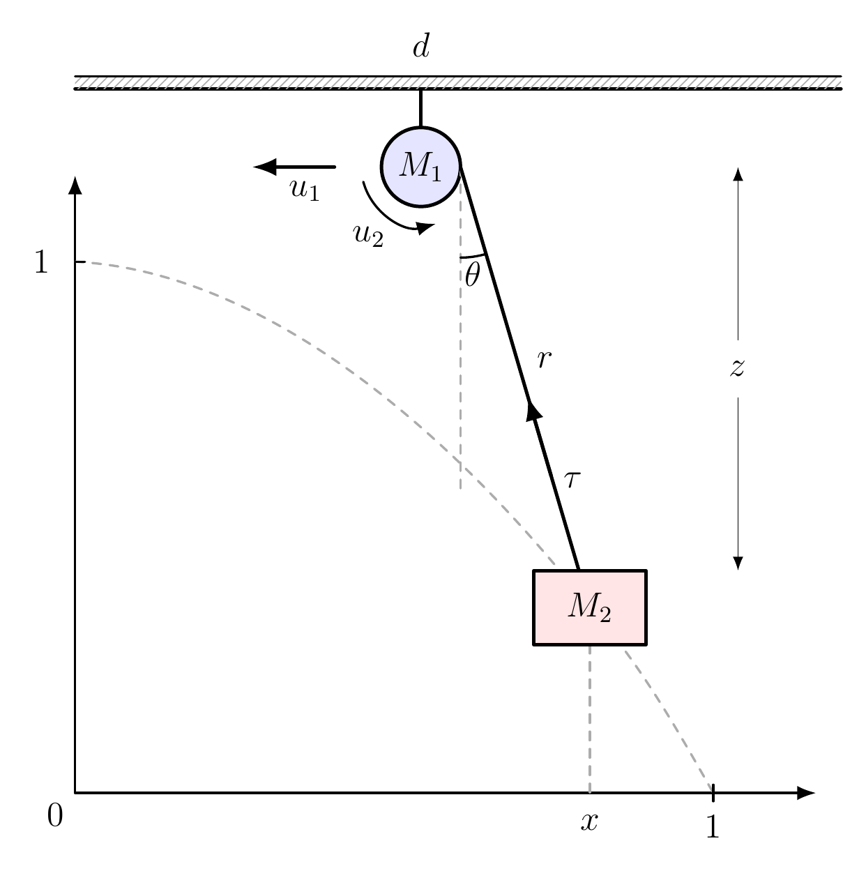
We consider an index-five DAE system that models the planar motion of a crane.
The goal is to determine the horizontal velocity u_1 and the angular velocity u_2 of a winch of mass M_1, so that the attached load of mass M_2 follows a prescribed path p_1(t) and p_2(t).

The DAEs, derived from Newton’s second law, are given by:

\left\{ \begin{aligned} x' &= v_x \\ z' &= v_z \\ d' &= v_d \\ r' &= v_r \\ M_2 v_x' &= -\tau \sin\theta \\ M_2 v_z' &= - \tau \cos\theta + m g\\ M_1 v_d' &= - C_1 v_d + u_1 + \tau\sin\theta \\ J v_r' &= - C_2 v_r - C_3 u_2 + C_3^2 \tau \\ x &= r\sin\theta + d \\ z & = r\cos\theta \\ x &= p_1(t) \\ z &= p_2(t) \end{aligned} \right.

where:

• (x, z) denotes the position of the load,
• \tau is the tension in the cable,
• \theta is the angle of the cable with the vertical,
• J is the moment of inertia of the winch,
• d is the position of the trolley,
• r is the length of the cable.

The constants satisfy C_1 > 0, C_2 > 0, C_3 > 0, g > 0, and m > 0.

Semi-Explicit Form

For the previous DAE system introduce dummy variables

• v_{x,\text{dot}}
• v_{z,\text{dot}}
• v_{d,\text{dot}}
• v_{r,\text{dot}}

and the system decomposes into differential (blue) and algebraic (red) components:

\left\{ \color{blue} \begin{aligned} x' &= v_x \\ z' &= v_z \\ d' &= v_d \\ r' &= v_r \\ v_x' &= v_{x,\text{dot}} \\ v_z' &= v_{z,\text{dot}} \\ v_d' &= v_{d,\text{dot}} \\ v_r' &= v_{r,\text{dot}} \end{aligned} \right. \quad \bigoplus \quad \left\{ \color{DarkRed} \begin{aligned} 0 &= M_2 v_{x,\text{dot}}+\tau \sin\theta && \text{(Constraint 1)}\\ 0 &= M_2 v_{z,\text{dot}}+\tau \cos\theta - m g && \text{(Constraint 2)}\\ 0 &= M_1 v_{d,\text{dot}}+C_1 v_d -u_1 -\tau\sin\theta && \text{(Constraint 3)}\\ 0 &= J v_{r,\text{dot}} +C_2 v_r + C_3 u_2 - C_3^2 \tau && \text{(Constraint 4)} \\ 0 &= r\sin\theta + d - x && \text{(Constraint 5)}\\ 0 &= r\cos\theta - z && \text{(Constraint 6)}\\ 0 &= p_1(t) - x && \text{(Constraint 7)}\\ 0 &= p_2(t) - z && \text{(Constraint 8)} \end{aligned} \right.

For this DAE we have:

• Differential variables: x, z, d, r, v_x, v_z, v_d, v_r .
• Algebraic variables:- v_{x,\text{dot}}, v_{z,\text{dot}}, v_{d,\text{dot}}, v_{r,\text{dot}}, u_1, u_2. \tau, \theta

The algebraic variables do not appears linearly in the constraints. In particular \theta appears nonlinear as \sin\theta and \cos\theta. Introducing the new dummy variable \theta_{\text{dot}} =\theta' we have for the differential part:

\left\{ \color{blue} \begin{aligned} x' &= v_x \\ z' &= v_z \\ d' &= v_d \\ r' &= v_r \\ v_x' &= v_{x,\text{dot}} \\ v_z' &= v_{z,\text{dot}} \\ v_d' &= v_{d,\text{dot}} \\ v_r' &= v_{r,\text{dot}} \\ \color{green}\theta' &\color{green}= \theta_{\text{dot}} \end{aligned} \right.

and now

• Differential variables: x, z, d, r, v_x, v_z, v_d, v_r, \theta.
• Algebraic variables:- v_{x,\text{dot}}, v_{z,\text{dot}}, v_{d,\text{dot}}, v_{r,\text{dot}}, u_1, u_2. \tau, \theta_{\text{dot}}

and not constraints are linear in the algebraic variables.

Reduction Procedure

We attempt to solve for v_{x,\text{dot}}, v_{z,\text{dot}}, v_{d,\text{dot}}, v_{r,\text{dot}}, but the system is not yet solvable explicitly. We proceed by differentiating.

Step 1: Differentiate algebraic constraints

We now differentiate the constraints to reduce the index. Here we want to differentiate only the algebraic equation that can reduce the index and do not introduce new differential equation. Here we want to avoid to introduce derivatove of the algebraic variable unless is strictly necessary.

We construct a dependency table to identify which constraints to differentiate:

\begin{array}{c|cccccccc} & v_{x,\text{dot}} & v_{z,\text{dot}} & v_{d,\text{dot}} & v_{r,\text{dot}} & \;\;u_1\;\; & \;\;u_2\;\; & \;\;\tau\;\; & \theta_{\text{dot}} \\[0.5em] \hline \\[0.1em] \text{(Constraint 1)} & 1 & 0 & 0 & 0 & 0 & 0 & 1 & 0 \\[0.5em] \text{(Constraint 2)} & 0 & 1 & 0 & 0 & 0 & 0 & 1 & 0 \\[0.5em] \text{(Constraint 3)} & 0 & 0 & 1 & 0 & 1 & 0 & 1 & 0 \\[0.5em] \text{(Constraint 4)} & 0 & 0 & 0 & 1 & 0 & 1 & 1 & 0 \\[0.5em] \text{(Constraint 5)} & 0 & 0 & 0 & 0 & 0 & 0 & 0 & 0 \\[0.5em] \text{(Constraint 6)} & 0 & 0 & 0 & 0 & 0 & 0 & 0 & 0 \\[0.5em] \text{(Constraint 7)} & 0 & 0 & 0 & 0 & 0 & 0 & 0 & 0 \\[0.5em] \text{(Constraint 8)} & 0 & 0 & 0 & 0 & 0 & 0 & 0 & 0 \end{array}

a 0 means the the function do not depend on the variable on the column. A 1 means dependence. The last four constraints are candidate for differentiation as it doesn’t introduce new algebraic variables. Differentiate thus the last constraints and substitute known variable in differential form using the ODE part

\begin{aligned} \text{(Constraint 5)}'\quad 0 & = v_r\sin\theta +r(\cos\theta)\theta_{\text{dot}}+v_d-v_x \\ \text{(Constraint 6)}'\quad 0 & = v_r\cos\theta - r(\sin\theta)\theta_{\text{dot}}-v_z \\ \text{(Constraint 7)}'\quad 0 & = p'_1(t) - v_x \\ \text{(Constraint 8)}'\quad 0 & = p'_2(t) - v_z \end{aligned}

so that algebraic parte of the DAE become:

\begin{aligned} & \left\{ \color{DarkRed} \begin{aligned} 0 &= M_2 v_{x,\text{dot}}+\tau \sin\theta && \text{(Constraint 1)}\\ 0 &= M_2 v_{z,\text{dot}}+\tau \cos\theta - m g && \text{(Constraint 2)}\\ 0 &= M_1 v_{d,\text{dot}}+C_1 v_d -u_1 -\tau\sin\theta && \text{(Constraint 3)}\\ 0 &= J v_{r,\text{dot}} +C_2 v_r + C_3 u_2 - C_3^2 \tau && \text{(Constraint 4)} \\ 0 &= v_r\sin\theta +r(\cos\theta)\theta_{\text{dot}}+v_d-v_x && \text{(Constraint 5)}'\\ 0 &= v_r\cos\theta - r(\sin\theta)\theta_{\text{dot}}-v_z && \text{(Constraint 6)}'\\ 0 &= p'_1(t) - v_x && \text{(Constraint 7)}'\\ 0 &= p'_2(t) - v_z && \text{(Constraint 8)}'\\ \end{aligned} \right. \\ & \left\{ \color{DarkGreen} \begin{aligned} 0 & = r\sin\theta + d - x &\qquad\qquad\qquad\quad& \text{(Constraint 5)}\\ 0 & = r\cos\theta - z && \text{(Constraint 6)}\\ 0 & = p_1(t) - x && \text{(Constraint 7)}\\ 0 & = p_2(t) - z && \text{(Constraint 8)} \end{aligned} \right. \end{aligned}

The red algebraic equations are the new algebraic equation after the derivation. The green algebraic equation is the hidden constraints that is removed from the DAE system but that is satisfied by choosing the right initial conditions.

The red part cannot determine the algebraic variable and must be differentiated again.

Step 2: Differentiate (again) the algebraic constraints

To find the right candidate(s) here we write a table of the dependencies

\begin{array}{c|cccccccc} & v_{x,\text{dot}} & v_{z,\text{dot}} & v_{d,\text{dot}} & v_{r,\text{dot}} & \;\;u_1\;\; & \;\;u_2\;\; & \;\;\tau\;\; & \theta_{\text{dot}} \\[0.5em] \hline \\[0.1em] \text{(Constraint 1)} & 1 & 0 & 0 & 0 & 0 & 0 & 1 & 0 \\[0.5em] \text{(Constraint 2)} & 0 & 1 & 0 & 0 & 0 & 0 & 1 & 0 \\[0.5em] \text{(Constraint 3)} & 0 & 0 & 1 & 0 & 1 & 0 & 1 & 0 \\[0.5em] \text{(Constraint 4)} & 0 & 0 & 0 & 1 & 0 & 1 & 1 & 0 \\[0.5em] \text{(Constraint 5)}' & 0 & 0 & 0 & 0 & 0 & 0 & 0 & 1 \\[0.5em] \text{(Constraint 6)}' & 0 & 0 & 0 & 0 & 0 & 0 & 0 & 1 \\[0.5em] \text{(Constraint 7)}' & 0 & 0 & 0 & 0 & 0 & 0 & 0 & 0 \\[0.5em] \text{(Constraint 8)}' & 0 & 0 & 0 & 0 & 0 & 0 & 0 & 0 \end{array}

The last two constraints are candidate for differentiation as it doesn’t introduce new algebraic variables. Differentiate thus the last constraints and substitute known variable in differential form using the ODE part

\begin{aligned} \text{(Constraint 7)}''\quad 0 & = p''_1(t) - v_{x,\text{dot}} \\ \text{(Constraint 8)}''\quad 0 & = p''_2(t) - v_{z,\text{dot}} \end{aligned}

and constraint part of the DAE become

\begin{aligned} & \left\{ \color{DarkRed} \begin{aligned} 0 &= M_2 v_{x,\text{dot}}+\tau \sin\theta && \text{(Constraint 1)}\\ 0 &= M_2 v_{z,\text{dot}}+\tau \cos\theta - m g && \text{(Constraint 2)}\\ 0 &= M_1 v_{d,\text{dot}}+C_1 v_d -u_1 -\tau\sin\theta && \text{(Constraint 3)}\\ 0 &= J v_{r,\text{dot}} +C_2 v_r + C_3 u_2 - C_3^2 \tau && \text{(Constraint 4)} \\ 0 &= v_r\sin\theta +r(\cos\theta)\theta_{\text{dot}}+v_d-v_x && \text{(Constraint 5)}'\\ 0 &= v_r\cos\theta - r(\sin\theta)\theta_{\text{dot}}-v_z && \text{(Constraint 6)}'\\ 0 &= p''_1(t) - v_{x,\text{dot}} && \text{(Constraint 7)}''\\ 0 &= p''_2(t) - v_{z,\text{dot}} && \text{(Constraint 8)}''\\ \end{aligned} \right. \\ & \left\{ \color{DarkGreen} \begin{aligned} 0 & = r\sin\theta + d - x &\qquad\qquad\qquad\quad & \text{(Constraint 5)}\\ 0 & = r\cos\theta - z && \text{(Constraint 6)}\\ 0 & = p_1(t) - x && \text{(Constraint 7)}\\ 0 & = p_2(t) - z && \text{(Constraint 8)} \\ 0 & = p'_1(t) - v_x && \text{(Constraint 7)}'\\ 0 & = p'_2(t) - v_z && \text{(Constraint 8)}'\\ \end{aligned} \right. \end{aligned}

Step 3: Differentiate (again) the algebraic constraints

To find the right candidate(s) here we write a table of the dependencies

\begin{array}{c|cccccccc} & v_{x,\text{dot}} & v_{z,\text{dot}} & v_{d,\text{dot}} & v_{r,\text{dot}} & \;\;u_1\;\; & \;\;u_2\;\; & \;\;\tau\;\; & \theta_{\text{dot}} \\[0.5em] \hline \\[0.1em] \text{(Constraint 1)} & 1 & 0 & 0 & 0 & 0 & 0 & 1 & 0 \\[0.5em] \text{(Constraint 2)} & 0 & 1 & 0 & 0 & 0 & 0 & 1 & 0 \\[0.5em] \text{(Constraint 3)} & 0 & 0 & 1 & 0 & 1 & 0 & 1 & 0 \\[0.5em] \text{(Constraint 4)} & 0 & 0 & 0 & 1 & 0 & 1 & 1 & 0 \\[0.5em] \text{(Constraint 5)}' & 0 & 0 & 0 & 0 & 0 & 0 & 0 & 1 \\[0.5em] \text{(Constraint 6)}' & 0 & 0 & 0 & 0 & 0 & 0 & 0 & 1 \\[0.5em] \text{(Constraint 7)}'' & 1 & 0 & 0 & 0 & 0 & 0 & 0 & 0 \\[0.5em] \text{(Constraint 8)}'' & 0 & 1 & 0 & 0 & 0 & 0 & 0 & 0 \end{array}

There are no constraints candidate for derivation. We can check if the constraints are enough to determine algebraic variable.

We use sprank of MATLAB to check if the matrix can be non singular.

sparsity_pattern = [...
1, 0, 0, 0, 0, 0, 1, 0; ...
0, 1, 0, 0, 0, 0, 1, 0; ...
0, 0, 1, 0, 1, 0, 1, 0; ...
0, 0, 0, 1, 0, 1, 1, 0; ...
0, 0, 0, 0, 0, 0, 0, 1; ...
0, 0, 0, 0, 0, 0, 0, 1; ...
1, 0, 0, 0, 0, 0, 0, 0; ...
0, 1, 0, 0, 0, 0, 0, 0; ...
];

fprintf('Estimated rank = %d\n', sprank(sparsity_pattern) );

> Estimated rank = 6

Matrix is not full rank. To continue the algorithm we can apply elimination to remove redundancy. First of all rewrite the constraint as a linear system

\underbrace{ \begin{bmatrix} M_{2} & 0 & 0 & 0 & 0 & 0 & \sin(\theta) & 0 \\ 0 & M_{2} & 0 & 0 & 0 & 0 & \cos(\theta) & 0 \\ 0 & 0 & M_{1} & 0 & -1 & 0 & -\sin(\theta) & 0 \\ 0 & 0 & 0 & J & 0 & C_{3} & -C_{3}^{2} & 0 \\ 0 & 0 & 0 & 0 & 0 & 0 & 0 & r \cos(\theta) \\ 0 & 0 & 0 & 0 & 0 & 0 & 0 & -r\sin(\theta) \\ -1 & 0 & 0 & 0 & 0 & 0 & 0 & 0 \\ 0 & -1 & 0 & 0 & 0 & 0 & 0 & 0 \end{bmatrix} }_{\bm{A}} \begin{pmatrix} v_{x,\text{dot}} \\ v_{z,\text{dot}} \\ v_{d,\text{dot}} \\ v_{r,\text{dot}}\\ u_1 \\ u_2 \\ \tau \\ \theta_{\text{dot}} \end{pmatrix} = \underbrace{ \begin{bmatrix} 0 \\ m g \\ -C_{1} v_{d} \\ -C_{2} v_{r} \\ v_{x}-v_{d}-v_{r}\sin(\theta) \\ v_{z} -v_{r}\cos(\theta) \\ -p''_{1}(t) \\ -p''_{2}(t) \end{bmatrix} }_{\bm{b}}

given \bm{L}_1 defined forward we have

\begin{aligned} \bm{L}_1 &= \begin{bmatrix} 1 & 0 & 0 & 0 & 0 & 0 & 0 & 0 \\ 0 & 1 & 0 & 0 & 0 & 0 & 0 & 0 \\ 0 & 0 & 1 & 0 & 0 & 0 & 0 & 0 \\ 0 & 0 & 0 & 1 & 0 & 0 & 0 & 0 \\ 0 & 0 & 0 & 0 & 1 & 0 & 0 & 0 \\ 0 & 0 & 0 & 0 & 0 & 1 & 0 & 0 \\ M_{2}^{-1} & 0 & 0 & 0 & 0 & 0 & 1 & 0 \\ 0 & M_{2}^{-1} & 0 & 0 & 0 & 0 & 0 & 1 \end{bmatrix} \\ \bm{L}_1\bm{A} &= \begin{bmatrix} M_{2} & 0 & 0 & 0 & 0 & 0 & \sin(\theta) & 0 \\ 0 & M_{2} & 0 & 0 & 0 & 0 & \cos(\theta) & 0 \\ 0 & 0 & M_{1} & 0 & -1 & 0 & -\sin(\theta) & 0 \\ 0 & 0 & 0 & J & 0 & C_{3} & -C_{3}^{2} & 0 \\ 0 & 0 & 0 & 0 & 0 & 0 & 0 & r\cos(\theta) \\ 0 & 0 & 0 & 0 & 0 & 0 & 0 & -r\sin(\theta) \\ 0 & 0 & 0 & 0 & 0 & 0 & M_2^{-1}\sin(\theta) & 0 \\ 0 & 0 & 0 & 0 & 0 & 0 & M_2^{-1}\cos(\theta) & 0 \end{bmatrix} \end{aligned}

given \bm{R}_1 defined forward we have \begin{aligned} \bm{R}_1 &= \begin{bmatrix} 1 & 0 & 0 & 0 & 0 & 0 & 0 & 0 \\ 0 & 1 & 0 & 0 & 0 & 0 & 0 & 0 \\ 0 & 0 & 1 & 0 & 0 & 0 & 0 & 0 \\ 0 & 0 & 0 & 1 & 0 & 0 & 0 & 0 \\ 0 & 0 & 0 & 0 & \cos(\theta) & -\sin(\theta) & 0 & 0 \\ 0 & 0 & 0 & 0 & \sin(\theta) & \cos(\theta) & 0 & 0 \\ 0 & 0 & 0 & 0 & 0 & 0 & \cos(\theta) & -\sin(\theta) \\ 0 & 0 & 0 & 0 & 0 & 0 & \sin(\theta) & \cos(\theta) \end{bmatrix} \\ \bm{R}_1\bm{L}_1\bm{A} &= \begin{bmatrix} M_{2} & 0 & 0 & 0 & 0 & 0 & \sin(\theta) & 0 \\ 0 & M_{2} & 0 & 0 & 0 & 0 & \cos(\theta) & 0 \\ 0 & 0 & M_{1} & 0 & -1 & 0 & -\sin(\theta) & 0 \\ 0 & 0 & 0 & J & 0 & C_{3} & -C_{3}^{2} & 0 \\ 0 & 0 & 0 & 0 & 0 & 0 & 0 & r \\ 0 & 0 & 0 & 0 & 0 & 0 & 0 & 0 \\ 0 & 0 & 0 & 0 & 0 & 0 & 0 & 0 \\ 0 & 0 & 0 & 0 & 0 & 0 & M_{2}^{-1} & 0 \end{bmatrix} \end{aligned}

\bm{R}_1\bm{L}_1\bm{A} have two rows zero, thus multiplying by \bm{R}_1\bm{L}_1 the constraints permits to find two algebraic constraints that can be derived.

\bm{R}_1\bm{L}_1 \begin{bmatrix} M_2 v_{x,\text{dot}}+\tau \sin\theta \\ M_2 v_{z,\text{dot}}+\tau \cos\theta - m g \\ M_1 v_{d,\text{dot}}+C_1 v_d -u_1 -\tau\sin\theta \\ J v_{r,\text{dot}} +C_2 v_r + C_3 u_2 - C_3^2 \tau \\ v_r\sin\theta +r(\cos\theta)\theta_{\text{dot}}+v_d-v_x \\ v_r\cos\theta - r(\sin\theta)\theta_{\text{dot}}-v_z \\ p''_1(t) - v_{x,\text{dot}} \\ p''_2(t) - v_{z,\text{dot}} \end{bmatrix} = \begin{bmatrix} M_2 v_{x,\text{dot}} + \tau \sin(\theta) \\ M_2 v_{z,\text{dot}}+ \tau \cos(\theta) - m g \\ M_{1} v_{d,\text{dot}}+C_{1} v_{d}-u_{1}-\tau\sin(\theta) \\ J v_{r,\text{dot}}+C_{2} v_{r}+C_{3} u_{2}-C_{3}^{2} \tau \\ v_{d}-v_{x}+ \cos(\theta)+r\theta_{\text{dot}}+ \sin(\theta) v_{z} \\ (v_{d}-v_{x}) \sin(\theta)-\cos(\theta) v_{z}+v_{r} \\ \cos(\theta) p''_{1}(t)-p''_{2}(t) \sin(\theta) +M_2^{-1}\sin(\theta) m g \\ \cos(\theta)p''_{2}(t)+p''_{1}(t) \sin(\theta) +M_2^{-1}(\tau -\cos(\theta)) m g \end{bmatrix}

Collecting the recombined constraints

\left\{ \color{BrickRed} \begin{aligned} 0 &= M_2 v_{x,\text{dot}}+\tau \sin\theta & \text{(C1)} \\ 0 &= M_2 v_{z,\text{dot}}+ \tau \cos(\theta) - m g & \text{(C2)} \\ 0 &= M_{1} v_{d,\text{dot}}+C_{1} v_{d}-u_{1}-\tau\sin(\theta) & \text{(C3)} \\ 0 &=J v_{r,\text{dot}}+C_{2} v_{r}+C_{3} u_{2}-C_{3}^{2} \tau & \text{(C4)} \\ 0 &=v_{d}-v_{x}+ \cos(\theta)+r\theta_{\text{dot}}+ \sin(\theta) v_{z} & \text{(C5)} \\ 0 &=(v_{d}-v_{x}) \sin(\theta)-\cos(\theta) v_{z}+v_{r} & \text{(C6)} \\ 0 &= \cos(\theta) p''_{1}(t)-p''_{2}(t) \sin(\theta) +M_2^{-1}\sin(\theta) m g & \text{(C7)} \\ 0 &=\cos(\theta)p''_{2}(t)+p''_{1}(t) \sin(\theta) +M_2^{-1}(\tau -\cos(\theta)) m g & \text{(C8)} \end{aligned} \right.

where we have renamed constraints because now are mixed by the multiplication of \bm{L}^{-1}. The constraints \text{(C6)} and \text{(C7)} can be derived.

\begin{aligned} \text{(C6)}' &= \left((v_{d}-v_{x}) \theta_{\text{dot}}-v_{z,\text{dot}}\right)\cos(\theta)+ \left(\theta_{\text{dot}}v_{z}+ v_{d,\text{dot}}-v_{x,\text{dot}}\right) \sin(\theta)+v_{r,\text{dot}} \\[0.5em] \text{(C7)}' &= p'''_{1}(t)\cos(\theta) -p'''_{2}(t)\sin(\theta) -\left(p''_{2}(t)\cos(\theta) +p''_{1}(t)\sin(\theta)\right) \theta_{\text{dot}}+ M_{2}^{-1} \theta_{\text{dot}}\cos(\theta) m g \end{aligned}

and the constraints and hidden constraints become:

\begin{aligned} & \left\{ \color{DarkRed} \begin{aligned} 0 &= M_2 v_{x,\text{dot}}+\tau \sin\theta && \text{(C1)} \\ 0 &=M_2 v_{z,\text{dot}}+ \tau \cos(\theta) - m g && \text{(C2)} \\ 0 &= M_{1} v_{d,\text{dot}}+C_{1} v_{d}-u_{1}-\tau\sin(\theta) && \text{(C3)} \\ 0 &=J v_{r,\text{dot}}+C_{2} v_{r}+C_{3} u_{2}-C_{3}^{2} \tau && \text{(C4)} \\ 0 &=v_{d}-v_{x}+ \cos(\theta)+r\theta_{\text{dot}}+ \sin(\theta) v_{z} && \text{(C5)} \\ 0 &= \left((v_{d}-v_{x}) \theta_{\text{dot}}-v_{z,\text{dot}}\right)\cos(\theta)+ \left(\theta_{\text{dot}}v_{z}+ v_{d,\text{dot}}-v_{x,\text{dot}}\right) \sin(\theta)+v_{r,\text{dot}} && \text{(C6)}' \\ 0 &= p'''_{1}(t)\cos(\theta) -p'''_{2}(t)\sin(\theta) -\left(p''_{2}(t)\cos(\theta) +p''_{1}(t)\sin(\theta)\right) \theta_{\text{dot}}+ M_{2}^{-1} \theta_{\text{dot}}\cos(\theta) m g && \text{(C7)}' \\ 0 &=\cos(\theta)p''_{2}(t)+p''_{1}(t) \sin(\theta) +M_2^{-1}(\tau -\cos(\theta) m g && \text{(C8)} \end{aligned} \right. \\ & \left\{ \color{DarkGreen} \begin{aligned} 0 & = r\sin\theta + d - x &\qquad & \text{(Constraint 5)}\\ 0 & = r\cos\theta - z && \text{(Constraint 6)}\\ 0 & = p_1(t) - x && \text{(Constraint 7)}\\ 0 & = p_2(t) - z && \text{(Constraint 8)} \\ 0 & = p'_1(t) - v_x && \text{(Constraint 7)}'\\ 0 & = p'_2(t) - v_z && \text{(Constraint 8)}'\\ 0 &=(v_{d}-v_{x}) \sin(\theta)-\cos(\theta) v_{z}+v_{r} && \text{(C6)} \\ 0 &= \cos(\theta) p''_{1}(t)-p''_{2}(t) \sin(\theta) +M_2^{-1}\sin(\theta) m g && \text{(C7)} \end{aligned} \right. \end{aligned}

Step 4: Differentiate the algebraic constraints?

To find the right candidate(s) here we write a table of the dependencies

\begin{array}{c|cccccccc} & v_{x,\text{dot}} & v_{z,\text{dot}} & v_{d,\text{dot}} & v_{r,\text{dot}} & \;\;u_1\;\; & \;\;u_2\;\; & \;\;\tau\;\; & \theta_{\text{dot}} \\[0.5em] \hline \\[0.1em] \text{(C1)} & 1 & 0 & 0 & 0 & 0 & 0 & 1 & 0 \\[0.5em] \text{(C2)} & 0 & 1 & 0 & 0 & 0 & 0 & 1 & 0 \\[0.5em] \text{(C3)} & 0 & 0 & 1 & 0 & 1 & 0 & 1 & 0 \\[0.5em] \text{(C4)} & 0 & 0 & 0 & 1 & 0 & 1 & 1 & 0 \\[0.5em] \text{(C5)} & 0 & 0 & 0 & 0 & 0 & 0 & 0 & 1 \\[0.5em] \text{(C6)}' & 1 & 1 & 1 & 1 & 0 & 0 & 0 & 1 \\[0.5em] \text{(C7)}' & 0 & 0 & 0 & 0 & 0 & 0 & 0 & 1 \\[0.5em] \text{(C8)} & 0 & 0 & 0 & 0 & 0 & 0 & 1 & 0 \end{array} There are no constraints candidate for derivation. We can check if the constraints are enough to determine algebraic variable.

We use sprank of MATLAB to check if the matrix can be non singular.

sparsity_pattern = [...
1, 0, 0, 0, 0, 0, 1, 0;...
0, 1, 0, 0, 0, 0, 1, 0;...
0, 0, 1, 0, 1, 0, 1, 0;...
0, 0, 0, 1, 0, 1, 1, 0;...
0, 0, 0, 0, 0, 0, 0, 1;...
1, 1, 1, 1, 0, 0, 0, 1;...
0, 0, 0, 0, 0, 0, 0, 1;...
0, 0, 0, 0, 0, 0, 1, 0;...
];

fprintf('Estimated rank = %d\n', sprank(sparsity_pattern) );

> Estimated rank = 7

the matrix is singular. Instead of apply LU try to combine \text{(C5)} and \text{(C7)}' to eliminate \theta_{\text{dot}}

\begin{aligned} \widetilde{\text{C7}} &= \text{(C5)} \left( M_2^{-1}mg\cos(\theta) - p''_{2}(t)\cos(\theta) - p''_{1}(t)\sin(\theta)\right)+ \text{(C7)}'r \\ &= \left( \cos(\theta)p'_1(t) -\cos(\theta) v_{d} -\sin(\theta)p'_2(t) \right) \left(\cos(\theta) p''_{2}(t) +\sin(\theta) p''_{1}(t)\right) \\ &+\left(\sin(\theta)p'''_{2}(t)-\cos(\theta) p'''_{1}(t)\right) r \\ & +M_2^{-1}\left( \cos(\theta) v_{d} -\cos(\theta) p'_1(t) +\sin(\theta)p'_2(t) \right) \cos(\theta) m g %& = %-\sin(\theta)^{2} p'_2(t)p''_{1}(t) \\ %& +\left( % \left( % M_2^{-1}p'_2(t) m g % -(v_{d}-p'_1(t)) p''_{1}(t) % -p'_2(t) p''_{2}(t) % \right) % \cos(\theta) % +rp'''_{2}(t) %\right) %\sin(\theta) %\\ % & % +\left( % (p'_1(t)-v_{d})p''_{2}(t) % +M_2^{-1}\left(v_{d}-p'_1(t)\right) m g % \right) % \cos(\theta)^{2}-r\cos(\theta)p'''_{1}(t) \end{aligned}

and

\begin{aligned} \widetilde{\text{C7}}' &= \left( M_2^{-1} \left( 2 p'_2\theta_{\text{dot}} - p''_1+ v_{d,\text{dot}} \right) m g + \left( p'_1-v_{d} \right) p'''_{2} +p''_1p''_{2} +2 \theta_{\text{dot}}(p'_1-v_{d}) p''_{1} -\left( 2 \theta_{\text{dot}}p'_2+v_{d,\text{dot}} \right) p''_{2} \right) \cos(\theta)^2 \\ &+\left( \left( M_2^{-1} \left( p''_2(t) + 2\theta_{\text{dot}}(p'_1(t)-v_{d}) \right) mg +( p'_1-v_{d})p'''_{1}-p'''_{2}p'_2+p''_{1}p''_1 -p''_{2}p''_2+ \left(-2 \theta_{\text{dot}}p'_2-v_{d,\text{dot}}\right) p''_{1} + \left(-2 \theta_{\text{dot}}p'_1+2 v_{d}\theta_{\text{dot}}\right)p''_{2} \right) \sin(\theta) +r\theta_{\text{dot}}p'''_{2}-rp''''_{1}-v_{r}p'''_{1} \right) \cos(\theta) \\ & +\left(-p'_2p'''_{1}-p''_2p''_{1} \right) \sin(\theta)^2+ \\ & \left(r \theta_{\text{dot}} p'''_{1}+rp''''_{2}+v_{r}p'''_{2}\right) \sin(\theta)-M_2^{-1}p'_2 \theta_{\text{dot}} m g +\left(-\theta_{\text{dot}} p'_1+v_{d}\theta_{\text{dot}}\right) p''_{1}+p''_{2}\theta_{\text{dot}}p'_2 \end{aligned}

TO BE COMPLETED

[1]

Xiaolin Qin, Juan Tang, Yong Feng, Bernhard Bachmann, and Peter Fritzson. 2016. Efficient index reduction algorithm for large scale systems of differential algebraic equations. Applied Mathematics and Computation 277, (2016), 10–22. https://doi.org/10.1016/j.amc.2015.11.091

[2]

Gunther Reissig, Wade Martinson, and Paul I. Barton. 2000. Differential-algebraic equations of index 1 may have an arbitrarily high structural index. SIAM Journal on Scientific Computing 21, 6 (2000), 1987–1990. https://doi.org/10.1137/S1064827599353853