
1 Laplace Transform definition
Visualization of the Laplace Transform
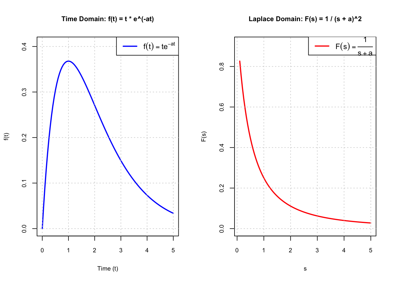
To visualize the effect of the Laplace Transform, consider the following example with an exponential function f(t) = e^{-at}. The Laplace Transform of this function is well-known:
f(t) = te^{-at} \quad \mapsto \quad \hat{f}(s) = \frac{1}{(s + a)^2}
Here’s a plot to illustrate the function and its Laplace Transform.
Code
# Define time and Laplace domain
t <- seq(0, 5, length=100)
a <- 1
f_t <- t * exp(-a * t)
s <- seq(0.1, 5, length=100)
F_s <- 1 / (s + a)^2

# Set up the plotting area with larger figure size
par(mfrow=c(1, 2), cex=0.8, cex.axis=0.8, cex.lab=0.8, cex.main=0.9)  # Two plots side by side

# Plot the time domain function
plot(t, f_t, type="l", col="blue", lwd=2,
     ylab="f(t)", xlab="Time (t)",
     main="Time Domain: f(t) = t * e^(-at)",
     ylim=c(0, max(f_t) * 1.1))  # Set y-limits for better visibility
grid()  # Add grid lines
legend("topright", legend=expression(f(t) == t * e^{-at}), col="blue", lwd=2)  # Add legend with LaTeX formatting

# Plot the Laplace Transform
plot(s, F_s, type="l", col="red", lwd=2,
     ylab="F(s)", xlab="s",
     main="Laplace Domain: F(s) = 1 / (s + a)^2",
     ylim=c(0, max(F_s) * 1.1))  # Set y-limits for better visibility
grid()  # Add grid lines

# Adjust y position for better vertical centering of the legend
legend("topright", legend=expression(F(s) == frac(1, s + a)), col="red", lwd=2, inset=c(0, -0.05)) # Add legend with LaTeX formatting and adjust position1.1 Transform Properties
The Laplace Transform possesses several important properties that facilitate calculations. One of the key properties to remember is that it acts as a linear operator:
Theorem 1.1 (linearity) The Laplace Transform exhibits a fundamental property known as linearity. For any functions
f(t) \mapsto \hat{f}(s) \quad \text{and} \quad g(t) \mapsto \hat{g}(s),
and for any real constants a, b \in \mathbb{R}, the linearity of the Laplace Transform can be expressed as follows:
h(t) := a \, f(t) + b \, g(t) \quad \mapsto \quad \hat{h}(s) := a \, \hat{f}(s) + b \, \hat{g}(s).
This means that the Laplace Transform of a linear combination of functions is equal to the same linear combination of their respective transforms.
Proof. The linearity property of the Laplace Transform can be demonstrated by applying the transform to a linear combination of two functions:
\mathscr{L}\left\{a \, f(t) + b \, g(t)\right\}(s) = \int_{0^-}^{\infty} \left( a \, f(t) + b \, g(t) \right) e^{-st} \, \mathrm{d}t.
Using the linearity of the integral, we can separate this into two distinct integrals:
\begin{aligned} &= a \int_{0^-}^{\infty} f(t) e^{-st} \, \mathrm{d}t + b \int_{0^-}^{\infty} g(t) e^{-st} \, \mathrm{d}t \\ &= a \, \hat{f}(s) + b \, \hat{g}(s). \end{aligned}
This confirms that the Laplace Transform of a linear combination of functions is equal to the same linear combination of their respective transforms.
However, it is important to note that not all functions allow for this property to hold. For specific cases where the integral may not converge, refer to Example Example 1.1 for further clarification.
Example 1.1 (Limits of intergral sequence) Consider a piecewise function f_n(t), parameterized by n, defined for t \geq 0 as follows:
f_n(t) = \begin{cases} nt & 0 \leq t \leq \frac{1}{n} \\ 2 - nt & \frac{1}{n} < t \leq \frac{2}{n} \\ 0 & \text{otherwise} \end{cases}
As n \to \infty, this function converges to f(t), which is zero everywhere:
f(t) = \lim_{n \to \infty} f_n(t).
To confirm this, we can compute the integral of f_n(t) over the interval [0, \infty):
F_n = \int_0^\infty f_n(t) \, \mathrm{d}t = \frac{1}{n} \quad \xrightarrow{n \to \infty} \quad 0.
Thus, as n \to \infty, the area under the curve tends to zero, consistent with the function becoming zero everywhere.
Misleading Intuition
At first glance, one might assume that the limit and the integral can be interchanged:
F = \int_0^\infty \lim_{n \to \infty} f_n(t) \, \mathrm{d}t = \lim_{n \to \infty} \int_0^\infty f_n(t) \, \mathrm{d}t.
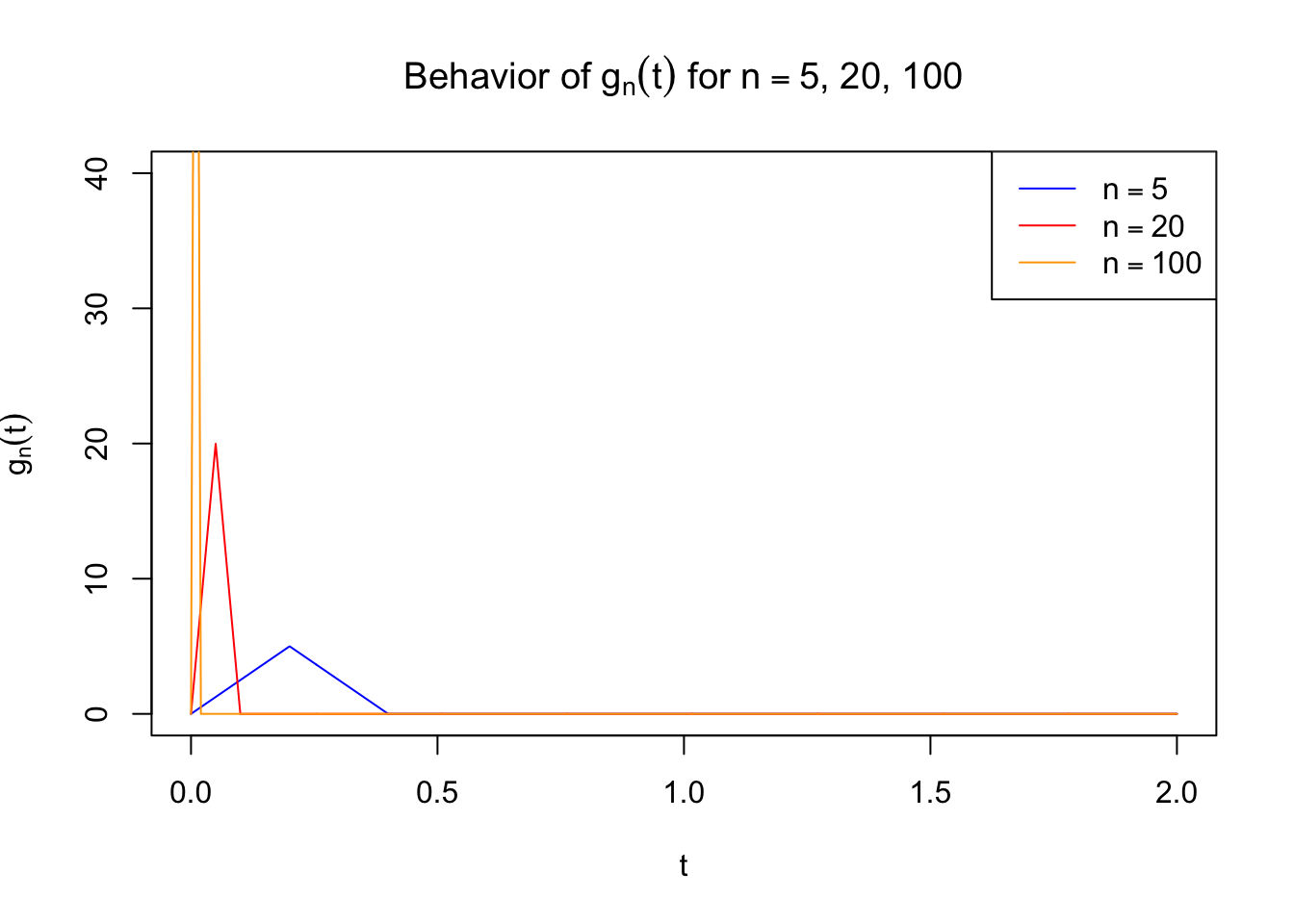
However, this is not always true. To illustrate this, consider another piecewise function g_n(t), defined as:
g_n(t) = \begin{cases} n^2 t & 0 \leq t < \frac{1}{n} \\ 2n - n^2 t & \frac{1}{n} < t < \frac{2}{n} \\ 0 & \text{otherwise} \end{cases}
Taking the limit as n \to \infty, we find that the function g(t) = \lim_{n \to \infty} g_n(t) = 0 everywhere. However, the computed area differs:
\lim_{n\to\infty} \int_0^\infty g_n(t)\, \mathrm{d}t = 1 \quad \neq \quad \int_0^\infty g(t)\, \mathrm{d}t = 0.
This demonstrates that, in general, the limit of the integral and the integral of the limit are not equivalent:
\lim_{n\to\infty} \int g_n(t) \mathrm{d}t \neq \int \lim_{n\to\infty} g_n(t) \mathrm{d}t.
Visualization
To further illustrate these concepts, we can visualize the behavior of f_n(t) and g_n(t) for various values of n. As n increases, observe how each function behaves and how their areas change.
Code
# Define function f_n(t)
fn <- function(t, n) {
  ifelse(t < 1/n, n * t, ifelse(t < 2/n, 2 - n * t, 0))
}

# Set up time axis
t <- seq(0, 2, length = 1000)

# Plot f_n(t) for n = 5, 20, and 100
plot(t, fn(t, 5), type = "l", col = "blue", ylim = c(0, 1.5),
     main = expression("Behavior of " * f[n](t) * " for " * n==5 * ", 20, 100"),
     ylab = expression(f[n](t)),
     xlab = expression(t))
lines(t, fn(t, 20), col = "red")
lines(t, fn(t, 100), col = "orange")

legend("topright",
       legend = c(expression(n==5), expression(n==20), expression(n==100)),
       col = c("blue", "red", "orange"), lty = 1)
Code
# Define function g_n(t)
gn <- function(t, n) {
  ifelse(t < 1/n, n^2 * t, ifelse(t < 2/n, 2 * n - n^2 * t, 0))
}

# Set up time axis
t <- seq(0, 2, length = 1000)

# Plot g_n(t) for n = 5, 20, and 100
plot(t, gn(t, 5), type = "l", col = "blue", ylim = c(0, 40),
     main = expression("Behavior of " * g[n](t) * " for " * n==5 * ", 20, 100"),
     ylab = expression(g[n](t)),
     xlab = expression(t))
lines(t, gn(t, 20), col = "red")
lines(t, gn(t, 100), col = "orange")

legend("topright",
       legend = c(expression(n==5), expression(n==20), expression(n==100)),
       col = c("blue", "red", "orange"), lty = 1)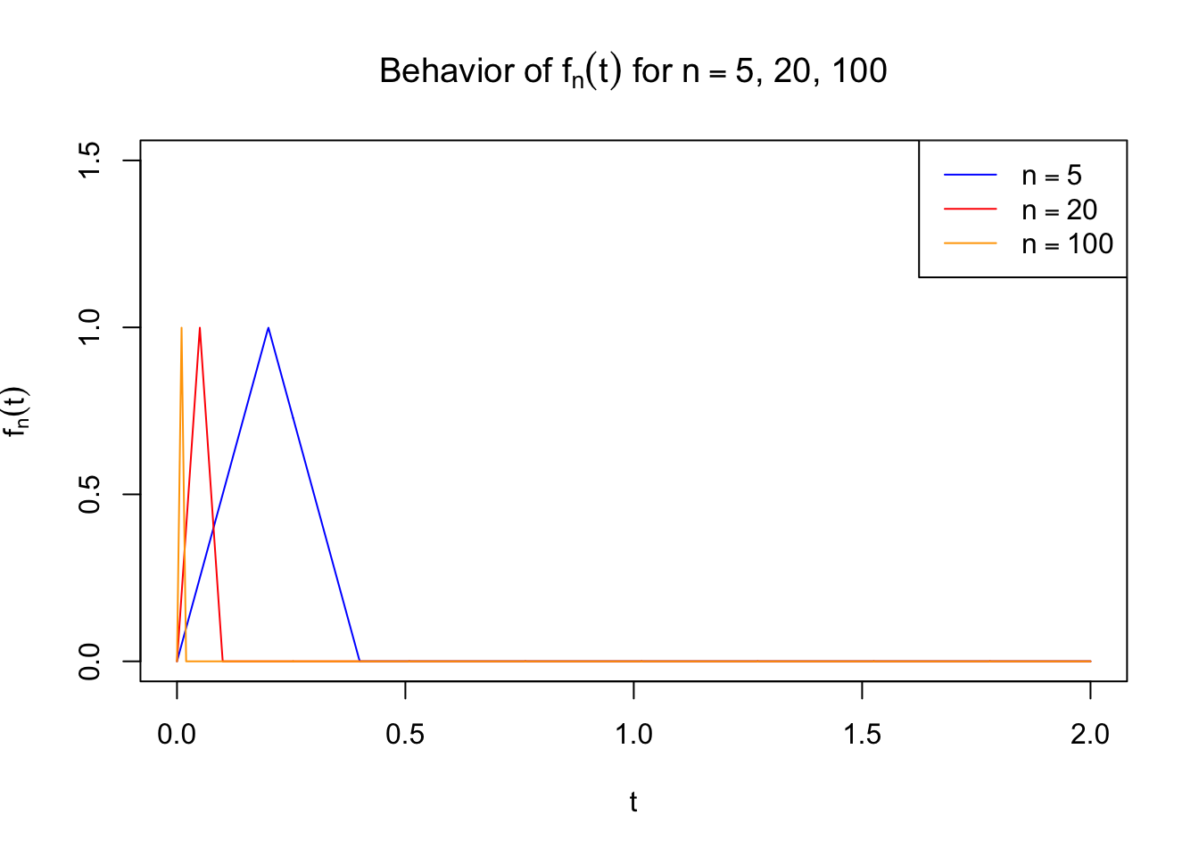
Scale Change and Translation Properties
In the study of Laplace transforms, the scaling and translation properties of the time axis play a significant role. These properties are essential for manipulating functions, allowing us to simplify their transformations and gain deeper insights into their behavior in the frequency domain.
Scaling of the Time Axis
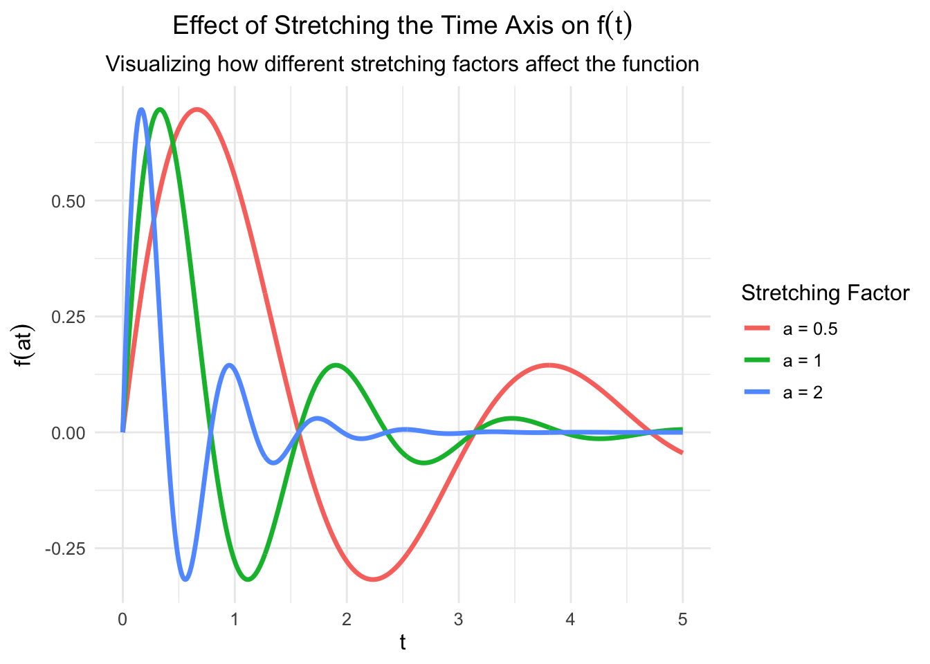
Theorem 1.2 (Stretching/Expanding the Time Axis) When we stretch or expand the time axis of a function f(t) by a factor a > 0, the corresponding Laplace Transform \hat{f}(s) is modified as follows:
f(at) \mapsto \frac{1}{a} \hat{f}\left(\frac{s}{a}\right).
Proof. The proof directly follows from the definition of the Laplace transform by applying a change of variables. Let at = z, which implies t = \frac{z}{a}:
\begin{aligned} \mathscr{L}\{f(at)\}(s) &= \int_{0^-}^{\infty} f(at)\, \mathrm{d}t \\ &= \int_{0^-}^{\infty} f(z) \, \mathrm{e}^{-s\frac{z}{a}} \, \frac{\mathrm{d}z}{a} \\ &= \frac{1}{a} \, \hat{f}\left(\frac{s}{a}\right) \end{aligned}
Code
library(ggplot2)

# Define the function f(t)
f <- function(t) {
  ifelse(t >= 0, exp(-t) * sin(4 * t), 0)  # Exponential decay for t >= 0
}

# Create a sequence of time values
t_vals <- seq(0, 5, by = 0.01)
a_values <- c(0.5, 1, 2)  # Different stretching factors
data <- data.frame()

# Create data for each stretching factor
for (a in a_values) {
  data <- rbind(data, data.frame(t = t_vals, f_t = f(a * t_vals), a = paste("a =", a)))
}

# Plot with ggplot2 using expression() for labels
ggplot(data, aes(x = t, y = f_t, color = a)) +
  geom_line(linewidth = 1.2) +
  labs(
    title = expression("Effect of Stretching the Time Axis on " * f(t)),
    subtitle = "Visualizing how different stretching factors affect the function",
    x = expression(t),
    y = expression(f(a*t)),
    color = "Stretching Factor"
  ) +
  theme_minimal() +
  theme(
    text = element_text(size=12),
    plot.title = element_text(hjust = 0.5, size=14),
    plot.subtitle = element_text(hjust = 0.5, size=12)
  )
Translation in the s and t axes
The translation property is a crucial aspect of Laplace transforms, affecting both the s axis and the t axis by a coefficient a > 0. These translations lead to the following relationships:
Theorem 1.3 (Translation in the s axes) \mathrm{e}^{at} f(t) \mapsto \hat{f}(s-a)
Proof. To prove the translation property in the s complex variable, we start with the Laplace Transform of the function e^{at} f(t):
\begin{aligned} \mathscr{L}\{\mathrm{e}^{at}f(t)\}(s) &= \int_{0^-}^{\infty} \mathrm{e}^{at} f(t) \mathrm{e}^{-st} \, \mathrm{d}t \\ &= \int_{0^-}^{\infty} f(t) \mathrm{e}^{(a-s)t} \, \mathrm{d}t \\ &= \hat{f}(s-a). \end{aligned}
This shows that multiplying by e^{at} translates the Laplace Transform along the s-axis.
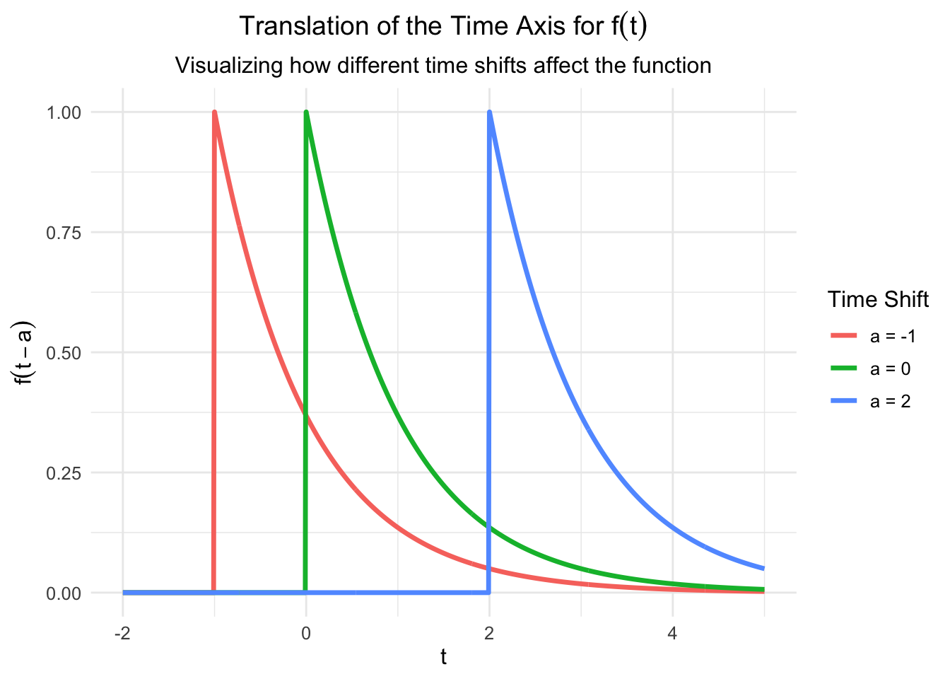
Theorem 1.4 (Translation in the t axes) f(t-a) \mapsto \mathrm{e}^{-as} \hat{f}(s)
Proof. For translation along the t-axis, we apply a change of variables with z = t - a:
\begin{aligned} \mathscr{L}\{f(t-a)\}(s) &= \int_{0^-}^{\infty} f(t-a) \, e^{-st} \, \mathrm{d}t \\ &= \int_{-a}^{\infty} f(z) e^{-s(z+a)}\, dz \\ &= e^{-as} \int_{0^-}^{\infty} f(z)e^{-sz}\, dz \\ &= e^{-as} \hat{f}(s). \end{aligned}
In this derivation, the first integral is effectively canceled because we typically assume that f(t) = 0 for t < 0. Therefore, this integral evaluates to zero.
Summary
These properties illustrate how translations in time and frequency domains impact the behavior of functions under Laplace transformations. The translation in the s-axis shifts the transform horizontally, while translation in the t-axis introduces an exponential decay factor.
Code
# Load necessary library
library(ggplot2)

# Define the function f(t) as before
f <- function(t) {
  ifelse(t >= 0, exp(-t), 0)  # Exponential decay for t >= 0
}

# Create a data frame for plotting with time shifts
t_vals <- seq(-2, 5, by = 0.01)
a_shifts <- c(-1, 0, 2)  # Different shifts in time
data_translation <- data.frame()

# Create data for each time shift
for (a in a_shifts) {
  data_translation <- rbind(
    data_translation,
    data.frame(t = t_vals, f_t = f(t_vals - a), a = paste("a =", a))
  )
}

# Plot with ggplot2 using expression() for math labels
ggplot(data_translation, aes(x = t, y = f_t, color = a)) +
  geom_line(linewidth = 1.2) +
  labs(
    title = expression("Translation of the Time Axis for " * f(t)),
    subtitle = "Visualizing how different time shifts affect the function",
    x = expression(t),
    y = expression(f(t - a)),
    color = "Time Shift"
  ) +
  theme_minimal() +
  theme(
    text = element_text(size=12),
    plot.title = element_text(hjust = 0.5, size=14),
    plot.subtitle = element_text(hjust = 0.5, size=12)
  )
1.2 Existence of the Laplace Transform
Not every function can be transformed using the Laplace operator \mathscr{L}. For instance, consider the function f(t) = \mathrm{e}^{t^2} cannot be transformd. In fadct, if we apply the Laplace transform to this function, we obtain the following integral:
\mathscr{L}\{\mathrm{e}^{t^2}\}(s) = \int_{0^-}^\infty \mathrm{e}^{t^2 - st} \, \mathrm{d}t = \int_{0^-}^T \mathrm{e}^{(t-s)t} \, \mathrm{d}t + \int_T^\infty \mathrm{e}^{(t-s)t} \, \mathrm{d}t.
If we choose a constant T > \Re(s) (the real part of s), we can observe that the second integral \int_T^\infty \mathrm{e}^{(t-s)t} \, \mathrm{d}t does not converge for any value s \in \mathbb{C}.
Proof. To prove this result, we start with the function f(t) = \mathrm{e}^{t^2}. If its Laplace transform exists (denoted by \hat{f}(s)), it must equal:
\hat{f}(s) = \lim_{M \to \infty} \int_{0^-}^M \mathrm{e}^{t(t-s)} \, \mathrm{d}t.
Since s is a complex variable, we express it as s = a + \mathrm{i}b, where a, b \in \mathbb{R} and \mathrm{i} = \sqrt{-1}. Substituting this into the Laplace transform expression gives:
\mathrm{e}^{t(t-a-\mathrm{i}b)} = \mathrm{e}^{t(t-a)} \mathrm{e}^{-\mathrm{i}bt}.
Using the De-Moivre formula 1 we rewrite the exponential with the imaginary term:
\mathrm{e}^{-\mathrm{i}bt} = \cos(bt) - \mathrm{i} \sin(bt).
Thus, the integral becomes:
\lim_{M \to \infty} \int_{0^-}^M \mathrm{e}^{t(t-a)} \left( \cos(bt) - \mathrm{i} \sin(bt) \right) \, \mathrm{d}t.
This expression can be split into real and imaginary parts:
Real part: R = \lim_{M \to \infty} \int_{0^-}^M \mathrm{e}^{t(t-a)} \cos(bt) \, \mathrm{d}t.
Imaginary part: I = \lim_{M \to \infty} \int_{0^-}^{M} \mathrm{e}^{t(t-a)} \sin(bt) \, \mathrm{d}t.
Focusing on the real part R, we note that it involves the product of a cosine function and an exponentially growing function. By analyzing this product at large values of t, we can see that the integral does not converge. To formalize this observation:
\begin{aligned} \int_0^{M + \Delta M} \mathrm{e}^{t(t-a)} \cos(bt) \, \mathrm{d}t &\geq \int_0^{M} \mathrm{e}^{t(t-a)} \cos(bt) \, \mathrm{d}t \\ &+ \mathrm{e}^{M(M-a)} \int_M^{M+\Delta M} \cos(bt) \, \mathrm{d}t. \end{aligned}
Since the exponential term \mathrm{e}^{t(t-a)} grows without bound as t increases, it follows that the integral does not converge. Consequently, we conclude that the Laplace transform for f(t) = \mathrm{e}^{t^2} does not exist.
Exponential Order Functions
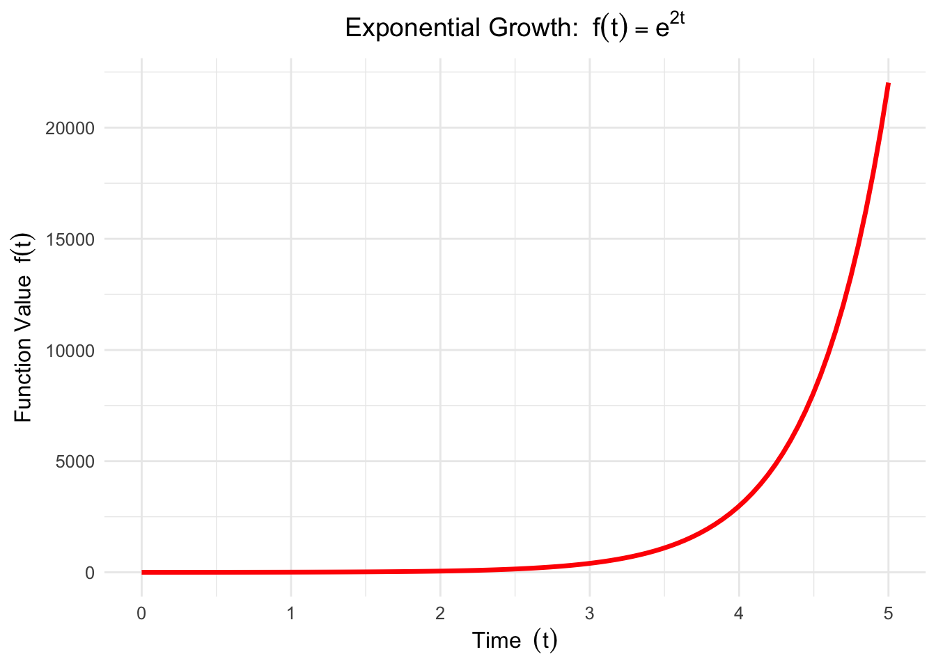
A function f(t) is said to be of exponential order if there exist constants M, N \in \mathbb{R} such that:
|f(t)| \leq M e^{Nt}
for all t \geq T, where T is a finite constant.
This definition implies that the growth of the function f(t) is bounded by an exponential function as t approaches infinity. Specifically, the term M e^{Nt} serves as an upper limit for the absolute value of f(t).
If a function is of exponential order, its Laplace transform exists in at least part of the complex plane. This means that we can find values of s for which the Laplace transform converges, providing valuable insights into the behavior of the function in the frequency domain.
Proof. To demonstrate that functions of exponential order always have a Laplace transform, we focus on the residual part of the integral from T to infinity:
\int_T^\infty |f(t)| \mathrm{e}^{-st} \, \mathrm{d}t.
Using the property |f(t)| \leq M \mathrm{e}^{Nt}, we can write:
\int_T^\infty |f(t)| \mathrm{e}^{-st} \, \mathrm{d}t \leq \int_T^\infty M \mathrm{e}^{Nt} \mathrm{e}^{-st} \, \mathrm{d}t = M \int_T^\infty \mathrm{e}^{(N - a)t} \, \mathrm{d}t,
where s = a + \mathrm{i}b and we focus on the real part a = \Re(s).
For convergence of the integral, we require a > N. Thus, if a > N, the term \mathrm{e}^{(N - a)t} tends to zero as t \to \infty, ensuring that the integral has a finite value.
Consequently, the domain of s for which the Laplace transform of an exponential order function exists is at least:
\Re(s) > N.
This result confirms that functions of exponential order have well-defined Laplace transforms within specific regions of the complex plane.
Code
# Load necessary library
library(ggplot2)

# Define the parameters for the plot
t <- seq(0, 5, length.out = 100)
N <- 2
f <- exp(N * t)

# Create a data frame for ggplot
data <- data.frame(t = t, f_t = f)

# Plot using ggplot2 for better aesthetics
ggplot(data, aes(x = t, y = f_t)) +
  geom_line(color = "red", linewidth = 1.2) +
  labs(
    title = expression("Exponential Growth: " ~ f(t) == e^{2*t}),
    x = expression("Time " ~ (t)),
    y = expression("Function Value " ~ f(t))
  ) +
  theme_minimal() +
  theme(
    text = element_text(size=12),
    plot.title = element_text(hjust = 0.5, size=14)
  )
According to the definition, we can also observe that the domain of the variable s for the Laplace transform of a function of exponential order is at least given by:
\forall s = a + \mathrm{i}b \in \mathbb{C}, \quad \text{such that} \quad a = \mathrm{Re}(s) \geq N.
This means that the real part of s must be greater than or equal to N for the Laplace transform to exist. In other words, the Laplace transform converges in the half-plane where the real part of s meets this condition.
2 Usage of the Laplace Transform
Consider the problem of solving the following differential equation:
\begin{cases} y'(t) = a\,y(t) + t \\ y(0) = 1 \end{cases}
Solving this equation in the time domain can be challenging. This is where the Laplace transform comes into play, allowing us to analyze the problem in the complex variable s. By applying the Laplace transform to the differential equation, we obtain:
\begin{aligned} \mathscr{L}\{y'(t)\}(s) & = \mathscr{L}\{a\,y(t) + t\}(s) \\ & = a \mathscr{L}\{y(t)\}(s) + \mathscr{L}\{t\}(s). \end{aligned}
At this point, we need to highlight an important Laplace transform property. This property states that the transform of the first derivative f'(t) of a function f(t) is given by:
f'(t) \mapsto s \hat{f}(s) - f(0^+),
where f(0^+) represents the value of the function f(t) at the origin of the time axis and corresponds to the initial (Cauchy) condition of the ordinary differential equation.
This property allows us to convert differential equations in the time domain into algebraic equations in the complex variable domain. Returning to our initial problem, we can rewrite the differential equation as:
s \hat{y}(s) - \underbrace{1}_{y(0^+)} = a \hat{y}(s) + \underbrace{\frac{1}{s^2}}_{\mathscr{L}\{t\}(s)}.
This simplifies to:
\hat{y}(s) = \dfrac{1 + \dfrac{1}{s^2}}{s - a}.
Example 2.1 (System of Ordinary Differential Equations) Consider the following system of two ordinary differential equations, subject to their initial conditions:
\begin{cases} x'(t) = y(t) + 1 \\ y'(t) = x(t) + \cos t \\ x(0) = 1 \\ y(0) = 1 \end{cases}
To solve this system, we can apply the Laplace transform to convert the equations into the complex variable domain. The Laplace transforms yield the following equations:
\begin{aligned} (i) & \quad \underbrace{s \tilde{x}(s) - x(0)}_{\mathscr{L}\{x'(t)\}(s)} &&= \tilde{y}(s) + \frac{1}{s} \\ (ii) & \quad \underbrace{s \tilde{y}(s) - y(0)}_{\mathscr{L}\{y'(t)\}(s)} &&= \tilde{x}(s) + \frac{1}{1+s^2} \end{aligned}
Knowing the initial conditions of the system allows us to express the system of functions \tilde{x} and \tilde{y} using matrix notation:
\underbrace{\begin{bmatrix} s & -1 \\ -1 & s \end{bmatrix}}_{A(s)} \begin{pmatrix} \tilde{x}(s) \\ \tilde{y}(s) \end{pmatrix} = \begin{pmatrix} 1 + \dfrac{1}{s} \\ \dfrac{1}{1+s^2} \end{pmatrix}
To find explicit values for \tilde{x}(s) and \tilde{y}(s), we can invert the matrix A(s):
\tilde{x}(s) = \dfrac{s + 1 - \dfrac{1}{1+s}}{s^2 - 1}, \qquad \tilde{y}(s) = \dfrac{\dfrac{s}{1+s} - 1 - \dfrac{1}{s}}{s^2 - 1}.
Example 2.2 (Computation of the Laplace Transform) Consider the ordinary differential equation:
\begin{cases} x'(t) + x(t) = \cos t \\ x(0) = 2 \end{cases}
To find the solution in the Laplace domain, we apply the Laplace transform operator \mathscr{L} to the entire equation. We utilize known transforms, specifically:
\begin{aligned} \mathscr{L}\{x(t)\}(s) &= \hat{x}(s), \\ \mathscr{L}\{x'(t)\}(s) &= s \hat{x}(s) - x(0), \\ \mathscr{L}\{\cos(t)\}(s) &= \frac{s}{s^2 + 1}. \end{aligned}
Applying the Laplace transform to the differential equation yields:
\mathscr{L}\{x'(t) + x(t)\}(s) = \mathscr{L}\{\cos t\}(s),
which translates to:
s \hat{x}(s) - 2 + \hat{x}(s) = \frac{s}{s^2 + 1}.
Now, we can combine terms to solve for \hat{x}(s):
(s + 1) \hat{x}(s) - 2 = \frac{s}{s^2 + 1}.
Rearranging gives us:
(s + 1) \hat{x}(s) = \frac{s}{s^2 + 1} + 2.
Finally, solving for \hat{x}(s) results in:
\hat{x}(s) = \frac{s}{(s+1)(s^2 + 1)} + \frac{2}{s+1} = \frac{2s^2 + s + 2}{(s+1)(s^2 + 1)}.
This expression represents the Laplace transform of the solution to the original ordinary differential equation.
\ \mathrm{e}^{A+\mathrm{i}B} = \mathrm{e}^A \mathrm{e}^{iB} = \mathrm{e}^A(\cos B +\mathrm{i}\sin B).↩︎