
11 Fundamental lemma of the calculus of variations
Considering the minimization of a a function
f:A\subseteq \Bbb{R}^n\mapsto \Bbb{R}
it has been shown that the first order necessary condition for a point \bm{x}^\star \in A to be a minimum point is that it’s gradient \nabla f(\bm{x}^\star) must be null. Similarly in calculus of variation it’s proven that the first order necessary condition for the optimality of the solution is that the first variation of the functional \mathcal{J} must be
\delta \mathcal{J}(x;\eta) = 0
for every admissible perturbation \eta(t).
In particular we define a perturbation \eta \in\Bbb{V} admissible for the functional \mathcal{J}:A\times A\mapsto \Bbb{R} respect to the function x(t) if it happens that x(\cdot) + \alpha \eta(\cdot) \in A for all value \alpha sufficiently close to 0.
Lemma 11.1 (Fundamental lemma of the calculus of variations) Given a function
f:[a,b]\mapsto \Bbb{R}, \qquad\textrm{(piecewise continuous)}
such that the integral satisfy \int_a^b f(x)\,g(x) \, \mathrm{d}x = 0 \tag{11.1}
for all g:[a,b] \mapsto \Bbb{R} smooth, i.e. g \in C^\infty([a,b]), with g^{(k)}(a) = g^{(k)}(b) = 0, \quad\forall k=0,1,2,3,\ldots
then f(x) is identically null.
Sign permanence
In order to later proof the fundamental lemma yet described, we have to remark the sign permanence that states:
Lemma 11.2 Given a function f:[a,b]\mapsto \Bbb{R} continuous such that f(c) >0, then there exists a \delta >0 such that
f(x) \geq \frac{f(c)}{2} \qquad \forall x \in [c-\delta,c+\delta]
Proof. The proof of this lemma can be done defining the parameter \epsilon = f(c) / 2; based on the assumption that f(x) is continuous, then exists a \delta>0 such that: |f(x) - f(c)| \leq \varepsilon = \frac{f(c)}{2} \qquad \forall |c-x|\leq \delta
Expanding the module operation the inequality becomes:
\begin{aligned} & -\frac{f(c)}{2} = - \epsilon \leq f(x)-f(c) \leq \epsilon = \frac{f(c)}{2} \\ &\implies \quad \underbrace{-\frac{f(c)}{2} + f(c) \leq f(x)}_{\frac{f(c)}{2} \leq f(x)} \leq f(c) + \frac{f(c)}{2} \end{aligned}
and so we prove the lemma of sign permanence. \square
Preparation of the proof of the fundamental lemma
The proof of the fundamental lemma of the calculus of variation can be done by contradiction.
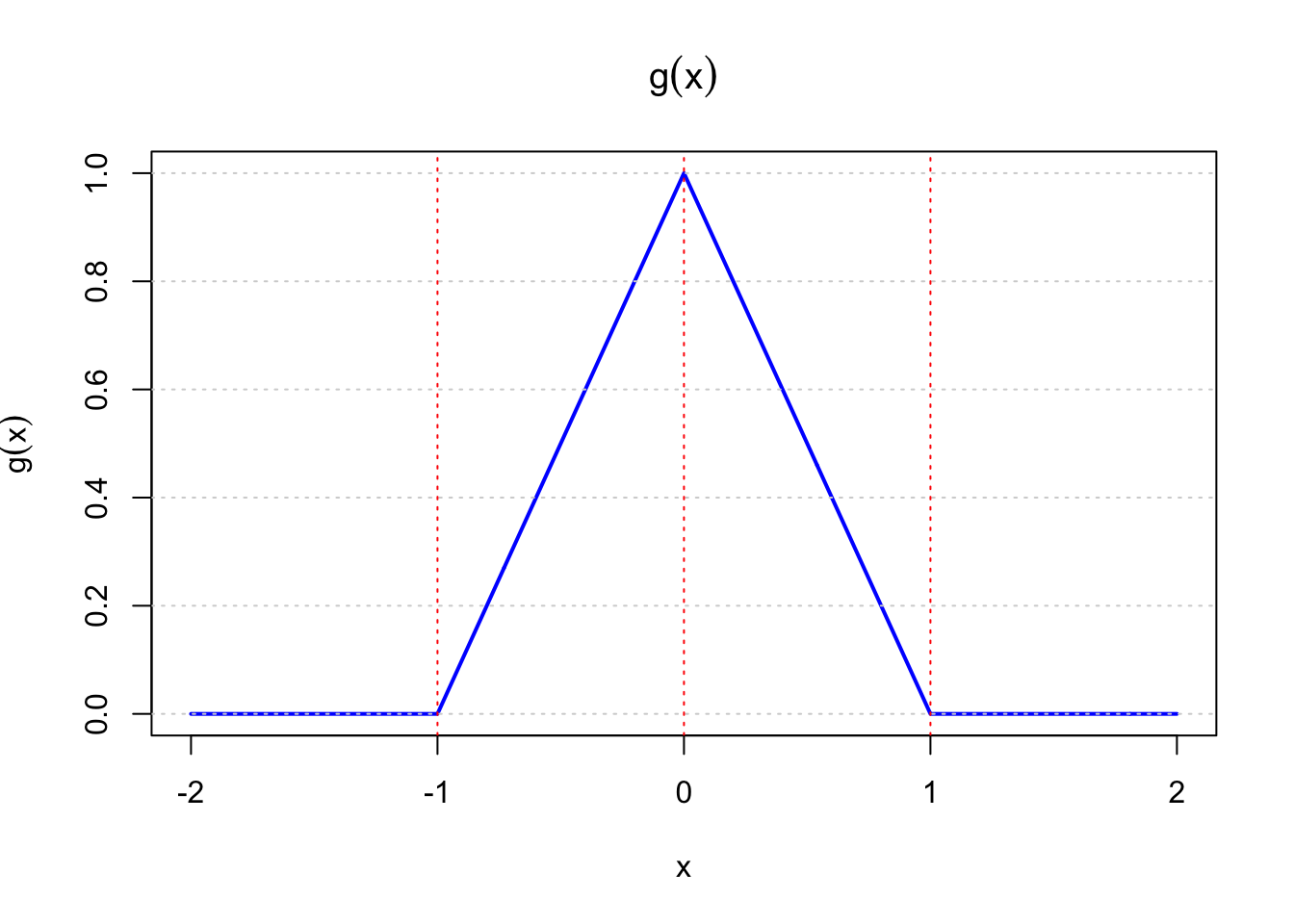
Let consider the integral Equation 11.1 and for the given function f, exists a point c such that f(c) > 0 (in general the proof can be done for f(c)\neq 0). From the sign permanence lemma we can state that exists an interval [c-\delta,c+\delta] such that f(x) \geq \frac{f(c)}{2 } \geq 0. Determining the function g as
g(x) = \begin{cases} \dfrac{x-(c-\delta)}{\delta} \qquad & x\in [c-\delta, c] \\ \dfrac{c-x+\delta}{\delta} & x\in[c,c+\delta] \\ 0 & \textrm{otherwise} \end{cases}
Code
g <- function(x, c, delta) {
  ifelse(x >= (c - delta) & x <= c,
         (x - (c - delta)) / delta,
         ifelse(x > c & x <= (c + delta),
                (c - x + delta) / delta,
                0))
}

# Grafico della funzione g
plot_g <- function(c, delta) {
  # Creare un vettore di valori x
  x_values <- seq(c - delta - 1, c + delta + 1, by = 0.01)

  # Valuta g per ogni x
  y_values <- g(x_values, c, delta)

  plot(x_values, y_values, type = "l", col = "blue",
       main = expression(g(x)),
       xlab = "x", ylab = expression(g(x)),
       ylim = c(0, 1), lwd = 2)

  # linee orizzontali e verticali
  abline(h = seq(0, 1, by = 0.2), col = "lightgray", lty = "dotted")
  abline(v = c(c - delta, c, c + delta), col = "red", lty = "dotted")
}

c <- 0
delta <- 1
plot_g(c, delta)Note that this function is continuous but g\notin C^\infty (later will be described a function that presents this feature). With this definition the integral \int_a^b fg\, \mathrm{d}x becomes
\int_{c-\delta}^{c+\delta} f(x)g(x)\, \mathrm{d}x \geq \frac{f(c)}{2} \int_{c-\delta}^{c+\delta} g(x)\, \mathrm{d}x \geq \frac{f(c)}{2}\frac \delta 2 > 0
We can clearly see that the integral \int_a^b fg\, \mathrm{d}x has a positive real value grater than zero that’s (considering that f has at least on point c such that f(c) >0) in contraposition with the initial request that the integral should have been zero evaluated.
To create a direction function g that’s in the set C^\infty we can use the function h(for whose those condition is demonstrated) as in Figure 11.2 defined as:
h(t) = \begin{cases} \mathrm{e}^{-1/t} \qquad & t > 0 \\ 0 & t\leq 0 \end{cases} \tag{11.2}
Code
# funzione h
h <- function(t) {
  ifelse(t > 0, exp(-1/t), 0)
}

# grafico della funzione h
plot_h <- function() {
  # Creare un vettore di valori t
  t_values <- seq(-1, 3, by = 0.01)

  # valori di h per ogni t
  y_values <- h(t_values)

  # il grafico
  plot(t_values, y_values, type = "l", col = "blue",
       main = expression(h(t)),
       xlab = "t", ylab = expression(h(t)),
       ylim = c(0, 1), lwd = 2)

  # linee orizzontali e verticali
  abline(h = seq(0, 1, by = 0.2), col = "lightgray", lty = "dotted")
}

plot_h()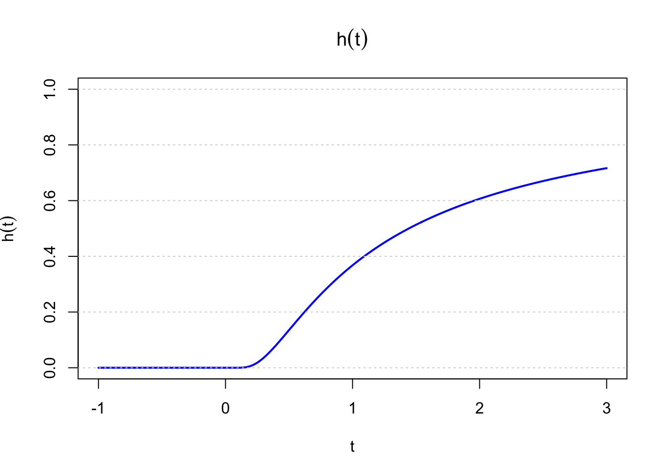
Code
# funzione h(t)
h <- function(t) {
  ifelse(t > 0, exp(-1/t), 0)
}

# derivate
h_prime <- function(t) {
  ifelse(t > 0, (exp(-1/t) / t^2), 0)
}

h_double_prime <- function(t) {
  ifelse(t > 0, (2 * exp(-1/t) / t^3 - exp(-1/t) / t^4), 0)
}

h_triple_prime <- function(t) {
  ifelse(t > 0, (6 * exp(-1/t) / t^4 - 3 * exp(-1/t) / t^5), 0)
}

# grafico con 4 riquadri
par(mfrow = c(2, 2), mar = c(3, 3, 2, 1))

# vettore di valori t
t_values <- seq(-1, 5, by = 0.01)

# valori di h(t) e delle derivate
h_values <- h(t_values)
h_prime_values <- h_prime(t_values)
h_double_prime_values <- h_double_prime(t_values)
h_triple_prime_values <- h_triple_prime(t_values)

# Plot di h(t)
plot(t_values, h_values, type = "l", col = "blue",
     main = expression(h(t)),
     ylim = c(0, 1), lwd = 2, axes = FALSE)
axis(2)
box()

# Plot della derivata prima
plot(t_values, h_prime_values, type = "l", col = "red",
     main = bquote({h^(1)}(t)),
     ylim = c(-0.5, 1), lwd = 2, axes = FALSE)
axis(2)
box()

# Plot della derivata seconda
plot(t_values, h_double_prime_values, type = "l", col = "green",
     main = bquote({h^(2)}(t)),
     ylim = c(-2.5, 1), lwd = 2, axes = FALSE)
axis(2)
box()

# Plot della derivata terza
plot(t_values, h_triple_prime_values, type = "l", col = "purple",
     main = bquote({h^(3)}(t)),
     ylim = c(-40, 2), lwd = 2, axes = FALSE)
axis(2)
box()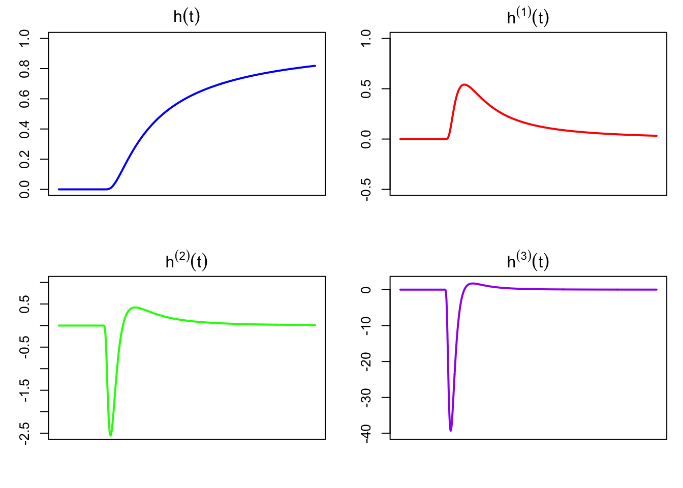
A way to create a function that presents a bell shape in the range [0,1] is by computing
g(t) := h(t) h(1-t)
how’s graph in the range [0,1] is similar to the one shown in figure Figure 11.4.
Code
# funzioni h(t) e g(t)
h <- function(t) { ifelse(t > 0, exp(-1/t), 0) }
g <- function(t) { h(t) * h(1 - t) }

# vettore di valori t
t_values <- seq(-1, 2, by = 0.01)

# valori di g(t)
g_values <- g(t_values)

# grafico di g(t)
plot(t_values, g_values, type = "l", col = "blue",
     main = expression("g(t) = h(t) . h(1 - t)"),
     xlab = "t", ylab = TeX("$g(t)$"),
     ylim = c(0, max(g_values)), lwd = 2)

grid()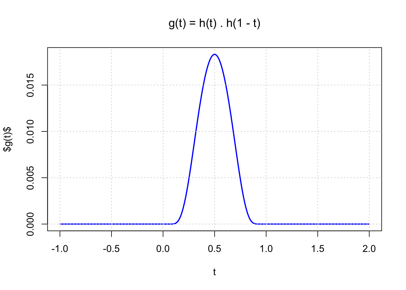
In particular, to demonstrate the fundamental lemma of the calculus of variations, we need to rescale the function g so that it has a bell shape centered at the point c with a bell width \delta. We consider the following formulation:
g(t) = K \, h\left(\frac{t - c + \delta}{2\delta}\right) h\left(\frac{\delta + c - t}{2\delta}\right)
where the constant K \in \mathbb{R} is chosen such that g(c) = 1 or \int_a^b g(x) \, \mathrm{d}x = 1.
In this case, we observe that:
g \in C^\infty(\Bbb{R}),
g(x) \geq 0 for all values of x, and specifically,
g(x) = 0 for all x \notin [c - \delta, c + \delta].
Lemma 11.1 can now be proven by contradiction.
Proof. As in the previous case, let us consider a function f(x) that is not identically zero. For this argument, we assume there exists at least one point c where f(c) > 0. By the sign permanence theorem, we can assert that:
f(x) \geq \frac{f(c)}{2} \qquad \forall x \in [c - \delta, c + \delta].
This inequality indicates that the function f(x) remains bounded away from zero within the interval [c - \delta, c + \delta].
Next, we examine the original integral \int_a^b fg\, \mathrm{d}x. Given our previous findings, we can conclude that this integral is not equal to zero. Specifically, we have:
\int_a^b f(x)g(x)\, \mathrm{d}x \geq \frac{f(c)}{2}\int_a^b g(x)\, \mathrm{d}x > 0.
Here, the term \frac{f(c)}{2} is positive, and since g(x) is non-negative for all x, the product \int_a^b f(x)g(x)\, \mathrm{d}x yields a positive value. This result constradict the assumption that f(x) in not identically zero. \square