
11 General Index Reduction
This chapter treats the general case. The object is a DAE written as
\bm E(\bm x,t)\,\dot{\bm x}=\bm G(\bm x,t),
which covers every semi-explicit system of Chapter 10 and the constant-coefficient systems of Chapter 7, and the goal is the one stated in Chapter 8, now for a state-dependent \bm E:
\text{DAE} \quad\xrightarrow{\ \text{differentiation}\ }\quad \text{ODE or index-1 DAE} \ \oplus\ \text{invariants.}
The algorithm is the same loop — separate, file, differentiate — but the separation now requires a state-dependent transformation, and constructing it is where the linear algebra enters.
11.1 The General Form \bm E(\bm x,t)\dot{\bm x}=\bm G(\bm x,t)
The semi-explicit transformation of Section 10.1 always produces a system of the shape
\bm E(\bm x,t)\,\dot{\bm x}=\bm G(\bm x,t), \qquad \bm E:\mathbb R^{n}\times\mathbb R\to\mathbb R^{n\times n}, \tag{11.1}
with \bm E=\begin{bmatrix}\bm I&\bm0\\\bm0&\bm0\end{bmatrix} in the semi-explicit case. There is no reason to keep that particular \bm E: the reduction algorithm below works for an arbitrary state- and time-dependent \bm E, and after one step the identity block is destroyed anyway. Taking Equation 11.1 as the object of study therefore costs nothing and covers all the semi-explicit cases of Section 10.2 at once, as well as the constant-coefficient DAE \bm E\dot{\bm x}=\bm A\bm x+\bm f(t) of Chapter 7.
Three cases, exactly parallel to the linear ones.
\bm E(\bm x,t) nonsingular. Then
\dot{\bm x}=\bm E(\bm x,t)^{-1}\bm G(\bm x,t)
is an ODE, or equivalently a DAE of index zero. In a code the inverse is never formed: one factorizes \bm E and solves at each evaluation.
\bm E(\bm x,t)\equiv\bm0. The system degenerates to the purely algebraic equation \bm0=\bm G(\bm x,t). Whether this can be turned into an ODE depends on \bm G: if \partial\bm G/\partial\bm x is nonsingular, differentiating
\frac{\mathrm d}{\mathrm dt}\bm G(\bm x,t) =\frac{\partial\bm G}{\partial\bm x}(\bm x,t)\,\dot{\bm x} +\frac{\partial\bm G}{\partial t}(\bm x,t)=\bm0
gives the ODE
\dot{\bm x} =-\left(\frac{\partial\bm G}{\partial\bm x}(\bm x,t)\right)^{-1} \frac{\partial\bm G}{\partial t}(\bm x,t), \tag{11.2}
whose solutions include those of \bm G=\bm0. As always, the original equation survives as an invariant and fixes the initial condition: \bm x(0) is not free but must solve \bm G(\bm x(0),0)=\bm0.
\bm E(\bm x,t) singular but not zero. This is the genuine DAE case and the subject of the rest of the chapter. Note that the rank of \bm E may depend on \bm x and t: a system can change index along a trajectory, and every statement below is local.
11.2 Separating the Algebraic Part with a Generalized LU
The reduction algorithm of Section 11.3 needs, at every step, a nonsingular \bm T(\bm x,t) that moves all the zero rows of \bm E(\bm x,t) to the bottom. This section constructs it, and the construction is nothing more than Gaussian elimination with pivoting applied to a possibly rectangular, possibly singular matrix.
LU with partial and full pivoting
For a nonsingular \bm A\in\mathbb R^{n\times n}, partial pivoting produces
\bm P\bm A=\bm L\bm U,
with \bm P a row permutation, \bm L unit lower triangular and \bm U upper triangular. Allowing column interchanges as well gives full pivoting,
\bm P\bm A\bm Q=\bm L\bm U , \tag{11.3}
with \bm Q a column permutation. The point for our purposes is that Equation 11.3 does not require \bm A to be square or nonsingular: the elimination of Appendix A stops when no nonzero pivot remains, and what it leaves is
\bm P\bm A\bm Q=\bm L\bm U, \qquad \bm U=\begin{pmatrix}\bm U_1&\bm N\\ \bm0&\bm0\end{pmatrix},
with \bm U_1\in\mathbb R^{k\times k} upper triangular and nonsingular, k=\operatorname{rank}\bm A. The precise statement, with the block factorization of both factors, is Theorem 8.1.
The form actually used: \bm P\bm A=\bm L\bm M
For index reduction the column permutation is a nuisance: permuting columns permutes the unknowns, and we want to touch only the equations. It can be absorbed.
Theorem 11.1 (Row-only rank-revealing factorization) Let \bm A\in\mathbb R^{m\times n} have rank k. Then there exist a permutation \bm P, a unit lower triangular \bm L and a matrix \bm M with
\boxed{\; \bm P\bm A=\bm L\bm M, \qquad \bm M=\begin{pmatrix}\bm M_1\\ \bm0\end{pmatrix}, \qquad \bm M_1\in\mathbb R^{k\times n}\ \text{of full row rank.} \;} \tag{11.4}
Proof. Apply Equation 11.3 to obtain \bm P\bm A\bm Q=\bm L\bm U. Since \bm Q is a permutation, \bm Q^{-1}=\bm Q^T and
\bm P\bm A=\bm L\bm U\bm Q^T=\bm L\bigl(\bm U\bm Q^T\bigr).
Right-multiplication by \bm Q^T permutes the columns of \bm U and therefore cannot create a nonzero entry in a zero row: the last m-k rows of \bm U\bm Q^T are still zero, and its first k rows have full row rank because \bm U_1 is nonsingular. Set \bm M=\bm U\bm Q^T. \square
The separator \bm L^{-1}\bm P
Apply Equation 11.4 to the matrix \bm E(\bm x,t) of Equation 11.1:
\bm P\bm E=\bm L\bm M \qquad\Longrightarrow\qquad \bm L^{-1}\bm P\,\bm E =\begin{pmatrix}\bm M_1\\ \bm0\end{pmatrix}. \tag{11.5}
Multiplying the DAE on the left by \bm L^{-1}\bm P therefore splits it into a differential and an algebraic block without changing its solution set:
\boxed{\; \bm T(\bm x,t)=\bm L(\bm x,t)^{-1}\bm P(\bm x,t) \quad\text{is the matrix that separates the algebraic part of a DAE.} \;} \tag{11.6}
This answers the question left open in Section 11.3. The factorization is recomputed at each reduction step, because \bm E changes; \bm L^{-1} is of course never formed, the product \bm L^{-1}\bm P\bm G being obtained by a forward substitution on the permuted right-hand side.
WarningThe permutation is not cosmetic
\bm P depends on \bm x and t through the pivot choice. A pivot that is nonzero but small makes \bm L badly conditioned, and the “zero” rows of \bm M are zero only to within a tolerance. The separation between differential and algebraic equations is therefore a numerical rank decision, with all that this implies: see Section 8.2.4. Near a point where the rank of \bm E changes, no factorization can make the choice for you.
11.3 Nonlinear Index Reduction
This tutorial explains how to compute the index of a non-linear DAE systematically.
General DAE
A general Differential-Algebraic equation (DAE) takes the form:
\bm{f}(\bm{x},\bm{x}^\prime,t) = \bm{0},
where
- \bm{x} represents the state variables
- \bm{x}^\prime denotes their derivatives with respect to time t
- \bm{f} is a system of equations involving both algebraic and differential components.
The defining characteristic of a DAE is that the Jacobian matrix
\frac{\partial \bm{f}(\bm{x},\bm{x}^\prime,t)}{\partial \bm{x}^\prime}
is singular, meaning that the system does not explicitly define all derivatives in terms of the state variables. This is in contrast to ordinary differential equations (ODEs), where the system can be solved explicitly for \bm{x}^\prime.
Semi-Explicit Form
Introducing the auxiliary variable \bm{y} = \bm{x}^\prime, the DAE can be rewritten as the system:
\left\{ \begin{aligned} \bm{x}^\prime &= \bm{y}, \\ \bm{0} &= \bm{f}(\bm{x},\bm{y},t). \end{aligned} \right.
This is a special case of the semi-explicit DAE of the form:
\left\{ \begin{aligned} \bm{x}^\prime &= \bm{g}(\bm{x},\bm{y},t), \\ \bm{0} &= \bm{f}(\bm{x},\bm{y},t), \end{aligned} \right.
where \bm{g} defines an explicit relationship for the differential variables.
Matrix Form
The semi-explicit DAE system can be expressed in a compact matrix form:
\underbrace{ \begin{pmatrix} \bm{I} & \bm{0} \\ \bm{0} & \bm{0} \end{pmatrix} }_{\bm{\mathcal{E}}(\bm{z},t)} \, \underbrace{ \begin{pmatrix} \bm{x}^\prime \\ \bm{y}^\prime \end{pmatrix} }_{\bm{\mathcal{z}}(t)} = \underbrace{ \begin{pmatrix} \bm{g}(\bm{x},\bm{y},t) \\ \bm{f}(\bm{x},\bm{y},t) \end{pmatrix} }_{\bm{\mathcal{G}}(\bm{z},t)}.
This formulation aligns with the general form of a DAE system:
\bm{\mathcal{E}}(\bm{z},t)\,\bm{z}(t) = \bm{\mathcal{G}}(\bm{z},t),
where \bm{\mathcal{E}}(\bm{z},t) is a singular matrix, reinforcing the differential-algebraic nature of the system.
Reduction Algorithm
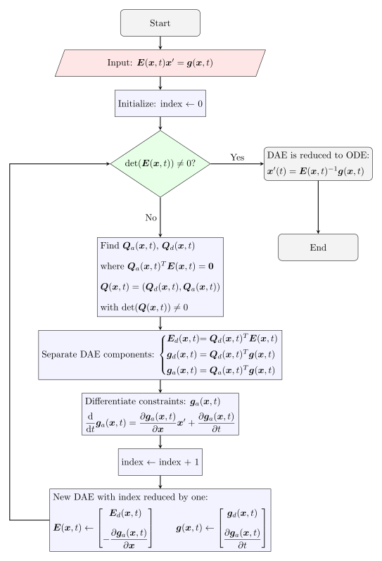
The differential index of a differential-algebraic equation (DAE) provides insight into the complexity of solving the system. The following steps outline an approach to determine the index and perform index reduction when necessary.
Step 1: Build the Matrix Form
A nonlinear DAE can be written as:
\bm{E}(\bm{x},t) \bm{x}^\prime = \bm{g}(\bm{x},t), \tag{11.7}
where:
- \bm{E}(\bm{x},t) is an n \times n matrix,
- \bm{x}(t) represents the state variables,
- \bm{x}^\prime is the time derivative of \bm{x},
- \bm{g}(\bm{x},t) is a given function.
This formulation allows us to analyze the structure of the system and determine if it contains purely algebraic constraints.
Step 2: Check Singularity
Compute the determinant:
- If \det(\bm{E}(\bm{x},t)) \neq 0, then \bm{E}(\bm{x},t) is invertible, and the system reduces to an ODE (index 0). Terminate the procedure.
- If \det(\bm{E}(\bm{x},t)) = 0, then \bm{E}(\bm{x},t) is singular, indicating that algebraic constraints are present. Proceed to the next step.
Remark 11.1 (Constant-Rank Assumption). We assume that \bm{E}(\bm{x},t) has constant rank in the domain of interest (\bm{x},t). If the rank varies, numerical methods must adapt accordingly, and the system’s index may change dynamically.
Step 3: Decompose the System
Determine the rank of \bm{E}(\bm{x},t), denoted as r = \operatorname{rank}(\bm{E}). Define:
A basis \bm{Q}_a(\bm{x},t) \in \mathbb{R}^{n \times (n-k)} for the null space \mathcal{N}(\bm{E}(\bm{x},t)^T), which identifies the algebraic constraints. This basis satisfies: \bm{E}(\bm{x},t)^T\bm{Q}_a(\bm{x},t) = \bm{0}, \quad \text{or equivalently,} \quad \bm{Q}_a(\bm{x},t)^T\bm{E}(\bm{x},t) = \bm{0}.
A matrix \bm{Q}_d(\bm{x},t) \in \mathbb{R}^{n \times k} that completes \bm{Q}_a(\bm{x},t) to a full basis, ensuring that: \bm{Q}(\bm{x},t) = \begin{pmatrix} \bm{Q}_d(\bm{x},t), \bm{Q}_a(\bm{x},t) \end{pmatrix} is non-singular.
By multiplying the original system by \bm{Q}(\bm{x},t)^T, we obtain:
Differential part: \color{blue} \bm{E}_d(\bm{x},t) \bm{x}^\prime = \bm{g}_d(\bm{x},t), where: \bm{E}_d(\bm{x},t) = \bm{Q}_d(\bm{x},t)^T \bm{E}(\bm{x},t), \quad \bm{g}_d(\bm{x},t) = \bm{Q}_d^T(\bm{x},t)\bm{g}(\bm{x},t).
Algebraic part: \color{blue} \bm{g}_a(\bm{x},t) = \bm{0}, where: \bm{g}_a(\bm{x},t) = \bm{Q}_a(\bm{x},t)^T\bm{g}(\bm{x},t). Since \bm{Q}_a(\bm{x},t)^T \bm{E}(\bm{x},t) = \bm{0}, no derivatives appear in this equation.
Step 4: Differentiate Constraints
The algebraic constraints must be differentiated to reveal hidden differential equations:
\frac{\mathrm{d}}{\mathrm{d}t} \bm{g}_a(\bm{x},t) = \bm{g}_a^t(\bm{x},t) + \bm{g}_a^x(\bm{x},t) \bm{x}^\prime(t) = \bm{0}.
Rewriting, the system becomes:
\begin{pmatrix} \bm{E}_d(\bm{x},t) \\ -\bm{g}_a^x(\bm{x},t) \end{pmatrix} \bm{x}^\prime = \begin{pmatrix} \bm{g}_d(\bm{x},t) \\ \bm{g}_a^t(\bm{x},t) \end{pmatrix}.
Defining:
\widetilde{\bm{E}}(\bm{x},t) = \begin{pmatrix} \bm{E}_d(\bm{x},t) \\ -\bm{g}_a^x(\bm{x},t) \end{pmatrix}, \quad \widetilde{\bm{g}}(\bm{x},t) = \begin{pmatrix} \bm{g}_d(\bm{x},t) \\ \bm{g}_a^t(\bm{x},t) \end{pmatrix},
we obtain a new DAE system:
\widetilde{\bm{E}}(\bm{x},t) \bm{x}^\prime = \widetilde{\bm{g}}(\bm{x},t).
Step 5: Repeat to Nonsingularity
Repeat Steps 2–4 until \widetilde{\bm{E}}(\bm{x},t) is invertible. The differentiation index is the number of times Step 4 is performed before reaching an ODE system.
11.4 Alternative Constructions and Which to Use
In the index reduction process, to separate the differential and algebraic components, we need to compute the kernel (null space) of \bm{E}, as it represents the algebraic constraints. There are different approaches available to compute it:
LU decomposition/factorization: a decomposition that factors a matrix A as the product of two matrices, \bm{A} = \bm{L}\bm{U}, where \bm{L} is a lower triangular matrix and \bm{U} is an upper triangular matrix;
Singular Value Decomposition (SVD): a factorization that factors a matrix as the product of three matrices \bm{A} = \bm{U} \bm{D} \bm{V}^T where the columns of \bm{U} and \bm{V} are orthonormal and the matrix \bm{D} is diagonal with positive real entries, to analyze matrix rank and separate the space into differential and algebraic components.
Kernel-Based Reduction
When the matrix \bm{E} is singular, there exists a nonzero vector \bm{v} \neq \bm{0} such that
\bm{E} \bm{v} = \bm{0}.
All such vectors form a linear subspace called the kernel of \bm{E}, denoted as \operatorname{Kernel}(\bm{E}). This subspace can be spanned by a set of basis vectors \{\bm{v}_i\}. Similarly, there exists a nonzero vector \bm{w} \neq \bm{0} such that
\bm{w}^T \bm{E} = \bm{0}^T,
which defines the kernel of the transpose of \bm{E}, denoted \operatorname{Kernel}(\bm{E}^T). This subspace is spanned by basis vectors \{\bm{w}_i\}.
We focus on the kernel of the transpose, cokernel,
\operatorname{Kernel}(\bm{E}^T) = \{\bm{w} \mid \bm{w}^T \bm{E} = \bm{0}\} = \operatorname{Span}\{\bm{w}_1, \bm{w}_2, \ldots, \bm{w}_p\} = \bm{K}.
Denoting \bm{K} = (\bm{w}_1, \bm{w}_2, \ldots, \bm{w}_p), it follows that
\bm{K}^T \bm{E} = \bm{0}.
If we can compute this kernel matrix \bm{K}(t,\bm{y}) for the time- and state-dependent matrix \bm{E}(t, \bm{y}), we can identify an invariant condition for the DAE.
Consider a general the DAE system Equation 11.7, and define
\bm{K}(t,\bm{y}) = \operatorname{Kernel}(\bm{E}(t,\bm{y})^T) = \operatorname{Cokernel}(\bm{E}).
Multiplying the original DAE by \bm{K}(t,\bm{y})^T, we get:
\bm{K}(t,\bm{y})^T \bm{E}(t,\bm{y}) \bm{y}^\prime = \bm{K}(t,\bm{y})^T \bm{G}(t,\bm{y}).
Since \bm{K}^T \bm{E} = \bm{0}, the left side vanishes, yielding
\bm{0} = \bm{K}(t,\bm{y})^T \bm{G}(t,\bm{y}).
This relation defines an invariant that the solution must satisfy.
Next, we extend the kernel matrix \bm{K}(t,\bm{y}) by finding a complementary matrix \bm{N}(t,\bm{y}) such that the combined matrix
\bm{M}(t,\bm{y}) = \begin{bmatrix} \bm{K}(t,\bm{y}) & \bm{N}(t,\bm{y}) \end{bmatrix}
is nonsingular (this process is often called the completion of the kernel).
Multiplying the original DAE by \bm{M}(t,\bm{y})^T separates the system into algebraic and differential parts:
\bm{M}(t,\bm{y})^T \bm{E}(t,\bm{y}) \bm{y}^\prime = \bm{M}(t,\bm{y})^T \bm{G}(t,\bm{y}),
which can be rewritten as
\begin{bmatrix} \bm{K}(t,\bm{y})^T \\ \bm{N}(t,\bm{y})^T \end{bmatrix} \bm{E}(t,\bm{y}) \bm{y}^\prime = \begin{bmatrix} \bm{K}(t,\bm{y})^T \\ \bm{N}(t,\bm{y})^T \end{bmatrix} \bm{G}(t,\bm{y}).
Manipulating the left side using \bm{K}^T \bm{E} = \bm{0} gives
\begin{bmatrix} \bm{0} \\ \bm{N}(t,\bm{y})^T \bm{E}(t,\bm{y}) \end{bmatrix} \bm{y}^\prime = \begin{bmatrix} \bm{K}(t,\bm{y})^T \bm{G}(t,\bm{y}) \\ \bm{N}(t,\bm{y})^T \bm{G}(t,\bm{y}) \end{bmatrix}.
Define
\bm{\tilde{G}}_1 = \bm{N}(t,\bm{y})^T \bm{G}(t,\bm{y}), \quad \bm{\tilde{G}}_2 = \bm{K}(t,\bm{y})^T \bm{G}(t,\bm{y}).
Differentiating \bm{\tilde{G}}_2 with respect to time,
\frac{d}{dt} \bm{\tilde{G}}_2(t,\bm{y}) = \frac{\partial \bm{\tilde{G}}_2(t,\bm{y})}{\partial t} + \frac{\partial \bm{\tilde{G}}_2(t,\bm{y})}{\partial \bm{y}} \bm{y}^\prime.
The reduced DAE system becomes
\begin{bmatrix} \bm{M}_1(t,\bm{y}) \\ - \frac{\partial \bm{\tilde{G}}_2(t,\bm{y})}{\partial \bm{y}} \end{bmatrix} \bm{y}^\prime = \begin{bmatrix} \bm{\tilde{G}}_1(t,\bm{y}) \\ \frac{\partial \bm{\tilde{G}}_2(t,\bm{y})}{\partial t} \end{bmatrix},
where \bm{M}_1(t,\bm{y}) = \bm{N}(t,\bm{y})^T \bm{E}(t,\bm{y}).
Thus, the DAE can be expressed as the system
\begin{cases} \bm{E}_2(t,\bm{y}) \bm{y}^\prime = \bm{G}_2(t,\bm{y}), \\ \bm{\tilde{G}}_2(t,\bm{y}) = \bm{0}, \end{cases}
with
\bm{E}_2(t,\bm{y}) = \begin{bmatrix} \bm{M}_1(t,\bm{y}) \\ - \frac{\partial \bm{\tilde{G}}_2(t,\bm{y})}{\partial \bm{y}} \end{bmatrix}, \quad \bm{G}_2(t,\bm{y}) = \begin{bmatrix} \bm{\tilde{G}}_1(t,\bm{y}) \\ \frac{\partial \bm{\tilde{G}}_2(t,\bm{y})}{\partial t} \end{bmatrix}.
This reduction process decreases the index of the DAE by one.
In summary, the algorithm proceeds as follows:
- Compute the kernel of \bm{E}^T.
- Complete the kernel to obtain a nonsingular matrix \bm{N}.
- Separate the algebraic and differential parts.
- Differentiate the algebraic constraints.
- Repeat as needed to reduce the index.
Kernel Methods
The goal is to find a matrix \mathbf{K} whose columns form a basis of \mathrm{Kernel}(\mathbf{E}^T), i.e., they satisfy
\mathbf{K}^T \mathbf{E} = \mathbf{0},
and such that the augmented matrix (\mathbf{K}, \mathbf{N}) is nonsingular (invertible), where \mathbf{N} complements \mathbf{K} to form a full-rank basis of the space.
Two classical methods to compute \mathbf{K} are described below.
LU Decomposition
The LU decomposition factorizes the matrix \mathbf{E} into a product of a lower triangular matrix \mathbf{L} and an upper trapezoidal matrix \mathbf{U}, up to row and column permutations given by permutation matrices \mathbf{P} and \mathbf{Q}:
\mathbf{P} \mathbf{E} \mathbf{Q} = \mathbf{L} \mathbf{U}.
Here, \mathbf{P} and \mathbf{Q} are chosen to ensure numerical stability and reveal the rank structure of \mathbf{E}.
Rearranging, the original matrix \mathbf{E} can be expressed as
\mathbf{E} = \mathbf{P}^T \mathbf{L} \mathbf{U} \mathbf{Q}^T.
Define
\mathbf{M} = \mathbf{U} \mathbf{Q}^T,
so that
\mathbf{E} = \mathbf{P}^T \mathbf{L} \mathbf{M}.
Because \mathbf{U} is upper trapezoidal, \mathbf{M} has a block structure of the form
\mathbf{M} = \begin{bmatrix} \mathbf{M}_1 \\ \mathbf{0} \end{bmatrix},
where \mathbf{M}_1 is full rank.
Multiplying both sides by \mathbf{L}^{-1} \mathbf{P}, we obtain
\mathbf{L}^{-1} \mathbf{P} \mathbf{E} = \mathbf{M} = \begin{bmatrix} \mathbf{M}_1 \\ \mathbf{0} \end{bmatrix}.
Now, by pre-multiplying with the block row selectors (\mathbf{I}, \mathbf{0}) and (\mathbf{0}, \mathbf{I}), where \mathbf{I} is the identity matrix and \mathbf{0} the zero matrix, we isolate the nonzero and zero parts respectively:
(\mathbf{I}, \mathbf{0}) \mathbf{L}^{-1} \mathbf{P} \mathbf{E} = \mathbf{M}_1,
(\mathbf{0}, \mathbf{I}) \mathbf{L}^{-1} \mathbf{P} \mathbf{E} = \mathbf{0}.
From this, we define the matrices \mathbf{K} and \mathbf{N} as
(\mathbf{K}, \mathbf{N}) := \mathbf{P}^T \mathbf{L}^{-T} \begin{bmatrix} \mathbf{0} & \mathbf{I} \\ \mathbf{I} & \mathbf{0} \end{bmatrix},
so that
\mathbf{N}^T = (\mathbf{I}, \mathbf{0}) \mathbf{L}^{-1} \mathbf{P}, \quad \text{and} \quad \mathbf{K}^T = (\mathbf{0}, \mathbf{I}) \mathbf{L}^{-1} \mathbf{P}.
By construction, \mathbf{K}^T \mathbf{E} = \mathbf{0}, and (\mathbf{K}, \mathbf{N}) is nonsingular. Thus, the LU decomposition provides a practical way to compute the kernel of \mathbf{E}.
Singular Value Decomposition
Another standard approach is to use the Singular Value Decomposition (SVD), which factorizes \mathbf{E} into orthogonal matrices \mathbf{U}, \mathbf{V}, and a diagonal matrix \mathbf{\Sigma}:
\mathbf{E} = \mathbf{U} \mathbf{\Sigma} \mathbf{V}^T,
where
\mathbf{U}^T \mathbf{U} = \mathbf{I}, \quad \mathbf{V}^T \mathbf{V} = \mathbf{I}, \quad \text{and} \quad \mathbf{\Sigma} = \mathrm{diag}(\sigma_1, \ldots, \sigma_r, 0, \ldots, 0).
Partitioning the matrices according to the rank r of \mathbf{E}, we write
\mathbf{E} = \left[ \begin{array}{c|c} \mathbf{U}_{11} & \mathbf{U}_{12} \\ \hline \mathbf{U}_{21} & \mathbf{U}_{22} \end{array} \right] \left[ \begin{array}{c|c} \mathbf{\Sigma}_r & \mathbf{0} \\ \hline \mathbf{0} & \mathbf{0} \end{array} \right] \left[ \begin{array}{c|c} \mathbf{V}_{11}^T & \mathbf{V}_{12}^T \\ \hline \mathbf{V}_{21}^T & \mathbf{V}_{22}^T \end{array} \right].
Multiplying both sides by \mathbf{U}^T and then selecting the lower block with (\mathbf{0}, \mathbf{I}), we get
(\mathbf{0}, \mathbf{I}) \mathbf{U}^T \mathbf{E} = (\mathbf{0}, \mathbf{I}) \left[ \begin{array}{c|c} \mathbf{\Sigma}_r & \mathbf{0} \\ \hline \mathbf{0} & \mathbf{0} \end{array} \right] \left[ \begin{array}{c|c} \mathbf{V}_{11}^T & \mathbf{V}_{12}^T \\ \hline \mathbf{V}_{21}^T & \mathbf{V}_{22}^T \end{array} \right] = \mathbf{0}.
This directly shows that the columns of (\mathbf{0}, \mathbf{I}) \mathbf{U}^T form a basis of the kernel of \mathbf{E}.
Defining
(\mathbf{K}, \mathbf{N}) = \mathbf{U} \begin{bmatrix} \mathbf{0} & \mathbf{I} \\ \mathbf{I} & \mathbf{0} \end{bmatrix},
we have
\mathbf{N}^T = (\mathbf{I}, \mathbf{0}) \mathbf{U}^T, \quad \text{and} \quad \mathbf{K}^T = (\mathbf{0}, \mathbf{I}) \mathbf{U}^T,
and thus \mathbf{K}^T \mathbf{E} = \mathbf{0}.
While the SVD method is robust and numerically stable, it is computationally more expensive than the LU approach and therefore less suited for large-scale or real-time applications. Also for symbolic computations, it is preferable to use LU decomposition.
A kernel-based separator
The factorization Equation 11.4 is not the only way to build the separator Equation 11.6. An equivalent construction starts from the left null space of \bm E,
\ker(\bm E^T)=\{\bm v:\bm v^T\bm E=\bm0\},
whose dimension is n-\operatorname{rank}\bm E. Let the columns of \bm K be a basis of \ker(\bm E^T), and let \bm L complete that basis to \mathbb R^{n}, so that
\bm S=\begin{pmatrix}\bm L^T\\ \bm K^T\end{pmatrix} \quad\text{is nonsingular.}
Then
\bm S\bm E =\begin{pmatrix}\bm L^T\bm E\\ \bm K^T\bm E\end{pmatrix} =\begin{pmatrix}\bm L^T\bm E\\ \bm0\end{pmatrix},
which is again the separation of Equation 11.5, with the algebraic equations in the bottom block.
WarningCorrect, but not recommended
The kernel construction is mathematically transparent and computationally awkward: it requires a basis of a null space and a completion of that basis to the whole space, both of which are more expensive and less stable than the elimination that produces Equation 11.4, and both of which must be recomputed at every reduction step and at every point (\bm x,t). Use it to understand what the separator does, not to compute it.
Which construction to use
Four routes to the same separation, in decreasing order of practicality.
| Construction | Cost | When it is the right choice |
|---|---|---|
| Elimination, \bm P\bm E=\bm L\bm M | \mathcal O(n^3), cheapest | the default for a numerical implementation |
| QR with column pivoting | \mathcal O(n^3), larger constant | when the rank decision is delicate and backward stability matters |
| SVD | \mathcal O(n^3), largest constant | when the numerical rank is genuinely ambiguous and must be decided by singular values |
| Kernel basis \bm S=(\bm L^T;\bm K^T) | highest | exposition only |
ImportantFor hand computation, do not use matrices at all
All of the above assume that the reduction is performed on the matrix \bm E(\bm x,t). For a system small enough to be treated by hand — which includes every example in this book and most textbook models — that is the wrong approach. It is faster and far less error-prone to write the system in the semi-explicit form of Section 10.1, identify the algebraic equations by inspection, differentiate them, and substitute the differential equations into the result. The pendulum reduction of Section 11.5 is carried out that way in four lines, whereas the matrix route requires assembling and factorizing a 5\times5 state-dependent matrix at each of three steps.
The matrix formulation earns its keep when the system is large, when the reduction must be automated, or when the rank of \bm E is not obvious — in other words, exactly when a human cannot do it by inspection.
11.5 Examples
A high-index chain
Consider the following DAE system:
\left\{ \begin{aligned} x_6'(t) + x_5(t) &= \sin t\\ x_5'(t) + x_4(t) &= \sin t\\ x_4'(t) + x_3(t) &= \sin t\\ x_3'(t) + x_2(t) &= \sin t\\ x_2'(t) + x_1(t) &= \sin t\\ x_6(t) &= \cos t \end{aligned} \right.
We define the variable vector and matrices:
\bm{Z} = \begin{pmatrix} x_1 \\[0.5em] x_2 \\[0.5em] x_3 \\[0.5em] x_4 \\[0.5em] x_5 \\[0.5em] x_6 \end{pmatrix}, \quad \bm{E}(\bm{Z},t) = \begin{pmatrix} 0 & 0 & 0 & 0 & 0 & 1 \\[0.5em] 0 & 0 & 0 & 0 & 1 & 0 \\[0.5em] 0 & 0 & 0 & 1 & 0 & 0 \\[0.5em] 0 & 0 & 1 & 0 & 0 & 0 \\[0.5em] 0 & 1 & 0 & 0 & 0 & 0 \\[0.5em] 0 & 0 & 0 & 0 & 0 & 0 \end{pmatrix}, \quad \bm{G}(\bm{Z},t) = \begin{pmatrix} \sin t - x_5(t)\\[0.5em] \sin t - x_4(t)\\[0.5em] \sin t - x_3(t)\\[0.5em] \sin t - x_2(t)\\[0.5em] \sin t - x_1(t)\\[0.5em] \cos t - x_6(t) \end{pmatrix}
So that the DAE reads:
\bm{E}(\bm{Z},t)\,\bm{Z}^\prime(t) = \bm{G}(\bm{Z},t)
Index Reduction
The table
\bm{T} = \left[\begin{array}{c|c} \bm{E}(\bm{Z},t) & \bm{G}(\bm{Z},t) \end{array} \right] = \left[ \begin{array}{rrrrrr|c} 0 & 0 & 0 & 0 & 0 & 1 & \sin t - x_5(t)\\[0.5em] 0 & 0 & 0 & 0 & 1 & 0 & \sin t - x_4(t)\\[0.5em] 0 & 0 & 0 & 1 & 0 & 0 & \sin t - x_3(t)\\[0.5em] 0 & 0 & 1 & 0 & 0 & 0 & \sin t - x_2(t)\\[0.5em] 0 & 1 & 0 & 0 & 0 & 0 & \sin t - x_1(t)\\[0.5em] 0 & 0 & 0 & 0 & 0 & 0 & \cos t - x_6(t) \end{array} \right]
is used to memorize the operation done on the DAE.
First Reduction
Reduce index by one
Let \color{blue}\text{[alg1]} = \cos t - x_6
Derive the constraint \text{[alg1]}
\frac{\mathrm{d}\text{[alg1]}}{\mathrm{d}t} = -\sin t - x'_6
rewrite the DAE
\bm{T}_1 = \left[ \begin{array}{rrrrrr|c} 0 & 0 & 0 & 0 & 0 & 1 & \sin t - x_5(t)\\[0.5em] 0 & 0 & 0 & 0 & 1 & 0 & \sin t - x_4(t)\\[0.5em] 0 & 0 & 0 & 1 & 0 & 0 & \sin t - x_3(t)\\[0.5em] 0 & 0 & 1 & 0 & 0 & 0 & \sin t - x_2(t)\\[0.5em] 0 & 1 & 0 & 0 & 0 & 0 & \sin t - x_1(t)\\[0.5em] 0 & 0 & 0 & 0 & 0 & 1 & -\sin t \end{array} \right]
Second Reduction
Reorder the equation
\bm{T}_2 = \left[ \begin{array}{rrrrrr|c} 0 & 1 & 0 & 0 & 0 & 0 & \sin t - x_1(t)\\[0.5em] 0 & 0 & 1 & 0 & 0 & 0 & \sin t - x_2(t)\\[0.5em] 0 & 0 & 0 & 1 & 0 & 0 & \sin t - x_3(t)\\[0.5em] 0 & 0 & 0 & 0 & 1 & 0 & \sin t - x_4(t)\\[0.5em] 0 & 0 & 0 & 0 & 0 & 1 & \sin t - x_5(t)\\[0.5em] 0 & 0 & 0 & 0 & 0 & 1 & -\sin t \end{array} \right]
Subtract row 5 to row 6
\bm{T}_3 = \left[ \begin{array}{rrrrrr|c} 0 & 1 & 0 & 0 & 0 & 0 & \sin t - x_1(t)\\[0.5em] 0 & 0 & 1 & 0 & 0 & 0 & \sin t - x_2(t)\\[0.5em] 0 & 0 & 0 & 1 & 0 & 0 & \sin t - x_3(t)\\[0.5em] 0 & 0 & 0 & 0 & 1 & 0 & \sin t - x_4(t)\\[0.5em] 0 & 0 & 0 & 0 & 0 & 1 & \sin t - x_5(t)\\[0.5em] 0 & 0 & 0 & 0 & 0 & 0 & x_5(t) - 2\sin t \end{array} \right]
found algebraic constraint
\color{blue}\text{[alg2]} = x_5 - 2 \sin t
Derive constraint \text{[alg2]}
\frac{\mathrm{d}\text{[alg2]}}{\mathrm{d}t} = x'_5 - 2 \cos t
so that
\bm{T}_4 = \left[ \begin{array}{rrrrrr|c} 0 & 1 & 0 & 0 & 0 & 0 & \sin t - x_1(t)\\[0.5em] 0 & 0 & 1 & 0 & 0 & 0 & \sin t - x_2(t)\\[0.5em] 0 & 0 & 0 & 1 & 0 & 0 & \sin t - x_3(t)\\[0.5em] 0 & 0 & 0 & 0 & 1 & 0 & \sin t - x_4(t)\\[0.5em] 0 & 0 & 0 & 0 & 0 & 1 & \sin t - x_5(t)\\[0.5em] 0 & 0 & 0 & 0 & 1 & 0 & 2 \cos t \end{array} \right]
Third Reduction
Subtract row 4 to row 6 \bm{T}_5 = \left[ \begin{array}{rrrrrr|c} 0 & 1 & 0 & 0 & 0 & 0 & \sin t - x_1(t)\\[0.5em] 0 & 0 & 1 & 0 & 0 & 0 & \sin t - x_2(t)\\[0.5em] 0 & 0 & 0 & 1 & 0 & 0 & \sin t - x_3(t)\\[0.5em] 0 & 0 & 0 & 0 & 1 & 0 & \sin t - x_4(t)\\[0.5em] 0 & 0 & 0 & 0 & 0 & 1 & \sin t - x_5(t)\\[0.5em] 0 & 0 & 0 & 0 & 0 & 0 & x_4(t) + 2 \cos t - \sin t \end{array} \right]
found algebraic constraint
\color{blue}\text{[alg3]} = x_4 + 2 \cos t - \sin t
Reduce index by one by deriving the constraint \text{[alg3]}
\frac{\mathrm{d}\text{[alg3]}}{\mathrm{d}t} = x'_4 - \cos t - 2\sin t
so that
\bm{T}_6 = \left[ \begin{array}{rrrrrr|c} 0 & 1 & 0 & 0 & 0 & 0 & \sin t - x_1(t)\\[0.5em] 0 & 0 & 1 & 0 & 0 & 0 & \sin t - x_2(t)\\[0.5em] 0 & 0 & 0 & 1 & 0 & 0 & \sin t - x_3(t)\\[0.5em] 0 & 0 & 0 & 0 & 1 & 0 & \sin t - x_4(t)\\[0.5em] 0 & 0 & 0 & 0 & 0 & 1 & \sin t - x_5(t)\\[0.5em] 0 & 0 & 0 & 1 & 0 & 0 & \cos t + 2\sin t \end{array} \right]
Fourth Reduction
Subtract row 3 to row 6
\bm{T}_7 = \left[ \begin{array}{rrrrrr|c} 0 & 1 & 0 & 0 & 0 & 0 & \sin t - x_1(t)\\[0.5em] 0 & 0 & 1 & 0 & 0 & 0 & \sin t - x_2(t)\\[0.5em] 0 & 0 & 0 & 1 & 0 & 0 & \sin t - x_3(t)\\[0.5em] 0 & 0 & 0 & 0 & 1 & 0 & \sin t - x_4(t)\\[0.5em] 0 & 0 & 0 & 0 & 0 & 1 & \sin t - x_5(t)\\[0.5em] 0 & 0 & 0 & 0 & 0 & 0 & \cos t + \sin t + x_3(t) \end{array} \right]
found algebraic constraint
\color{blue}\text{[alg4]} = x_3 + \sin t + \cos t
Reduce index by one by deriving the constraint \text{[alg4]}
\frac{\mathrm{d}\text{[alg4]}}{\mathrm{d}t} = x'_3 + \cos t - \sin t
so that
\bm{T}_8 = \left[ \begin{array}{rrrrrr|c} 0 & 1 & 0 & 0 & 0 & 0 & \sin t - x_1(t)\\[0.5em] 0 & 0 & 1 & 0 & 0 & 0 & \sin t - x_2(t)\\[0.5em] 0 & 0 & 0 & 1 & 0 & 0 & \sin t - x_3(t)\\[0.5em] 0 & 0 & 0 & 0 & 1 & 0 & \sin t - x_4(t)\\[0.5em] 0 & 0 & 0 & 0 & 0 & 1 & \sin t - x_5(t)\\[0.5em] 0 & 0 & 1 & 0 & 0 & 0 & \sin t - \cos t \end{array} \right]
Fifth Reduction
Subtract row 2 to row 6
\bm{T}_9 = \left[ \begin{array}{rrrrrr|c} 0 & 1 & 0 & 0 & 0 & 0 & \sin t - x_1(t)\\[0.5em] 0 & 0 & 1 & 0 & 0 & 0 & \sin t - x_2(t)\\[0.5em] 0 & 0 & 0 & 1 & 0 & 0 & \sin t - x_3(t)\\[0.5em] 0 & 0 & 0 & 0 & 1 & 0 & \sin t - x_4(t)\\[0.5em] 0 & 0 & 0 & 0 & 0 & 1 & \sin t - x_5(t)\\[0.5em] 0 & 0 & 0 & 0 & 0 & 0 & x_2(t) - \cos t \end{array} \right]
found algebraic constraint
\color{blue}\text{[alg5]} = x_2 - \cos t
Reduce index by one by deriving the constraint \text{[alg5]} \frac{\mathrm{d}\text{[alg5]}}{\mathrm{d}t} = x'_2 + \sin t
so that
\bm{T}_{10} = \left[ \begin{array}{rrrrrr|c} 0 & 1 & 0 & 0 & 0 & 0 & \sin t - x_1(t)\\[0.5em] 0 & 0 & 1 & 0 & 0 & 0 & \sin t - x_2(t)\\[0.5em] 0 & 0 & 0 & 1 & 0 & 0 & \sin t - x_3(t)\\[0.5em] 0 & 0 & 0 & 0 & 1 & 0 & \sin t - x_4(t)\\[0.5em] 0 & 0 & 0 & 0 & 0 & 1 & \sin t - x_5(t)\\[0.5em] 0 & 1 & 0 & 0 & 0 & 0 & -\sin t \end{array} \right]
Sixth Reduction
Subtract row 1 to row 6
\bm{T}_{11} = \left[ \begin{array}{rrrrrr|c} 0 & 1 & 0 & 0 & 0 & 0 & \sin t - x_1(t)\\[0.5em] 0 & 0 & 1 & 0 & 0 & 0 & \sin t - x_2(t)\\[0.5em] 0 & 0 & 0 & 1 & 0 & 0 & \sin t - x_3(t)\\[0.5em] 0 & 0 & 0 & 0 & 1 & 0 & \sin t - x_4(t)\\[0.5em] 0 & 0 & 0 & 0 & 0 & 1 & \sin t - x_5(t)\\[0.5em] 0 & 0 & 0 & 0 & 0 & 0 & x_1(t) - 2\sin t \end{array} \right]
found algebraic constraint
\color{blue}\text{[alg6]} = x_1 - 2\sin t
Reduce index y one by deriving the constraint \text{[alg6]}
\frac{\mathrm{d}\text{[alg6]}}{\mathrm{d}t} = x_1' - 2\cos t
so that
\bm{T}_{12} = \left[ \begin{array}{rrrrrr|c} 0 & 1 & 0 & 0 & 0 & 0 & \sin t - x_1(t)\\[0.5em] 0 & 0 & 1 & 0 & 0 & 0 & \sin t - x_2(t)\\[0.5em] 0 & 0 & 0 & 1 & 0 & 0 & \sin t - x_3(t)\\[0.5em] 0 & 0 & 0 & 0 & 1 & 0 & \sin t - x_4(t)\\[0.5em] 0 & 0 & 0 & 0 & 0 & 1 & \sin t - x_5(t)\\[0.5em] 1 & 0 & 0 & 0 & 0 & 0 & 2\cos t \end{array} \right]
ODE Form
Now matrix is non-singular ans the resulting ODE is
\left\{ \begin{aligned} x'_1(t) & = 2\cos t \\ x'_2(t) & = \sin t - x_1(t) \\ x'_3(t) & = \sin t - x_2(t) \\ x'_4(t) & = \sin t - x_3(t) \\ x'_5(t) & = \sin t - x_4(t) \\ x'_6(t) & = \sin t - x_5(t) \end{aligned} \right.
with invariants (or hidden constraints)
\begin{aligned} \color{blue}\text{[alg1]} &= \cos t - x_6\\ \color{blue}\text{[alg2]} &= x_5 - 2\sin t\\ \color{blue}\text{[alg3]} &= x_4 + 2\cos t - \sin t\\ \color{blue}\text{[alg4]} &= x_3 + \sin t + \cos t \\ \color{blue}\text{[alg5]} &= x_2 - \cos t \\ \color{blue}\text{[alg6]} &= x_1 - 2\sin t \end{aligned}
Notice that from the invariants we can deduce
\begin{aligned} x_1(t) & = 2\sin t, \\ x_2(t) & = \cos t, \\ x_3(t) & = -\sin t -\cos t \\ x_4(t) & = \sin t - 2\cos t, \\ x_5(t) & = 2\sin t, \\ x_6(t) & = \cos t \end{aligned}
and the general solution in determined without fixing any initial value.
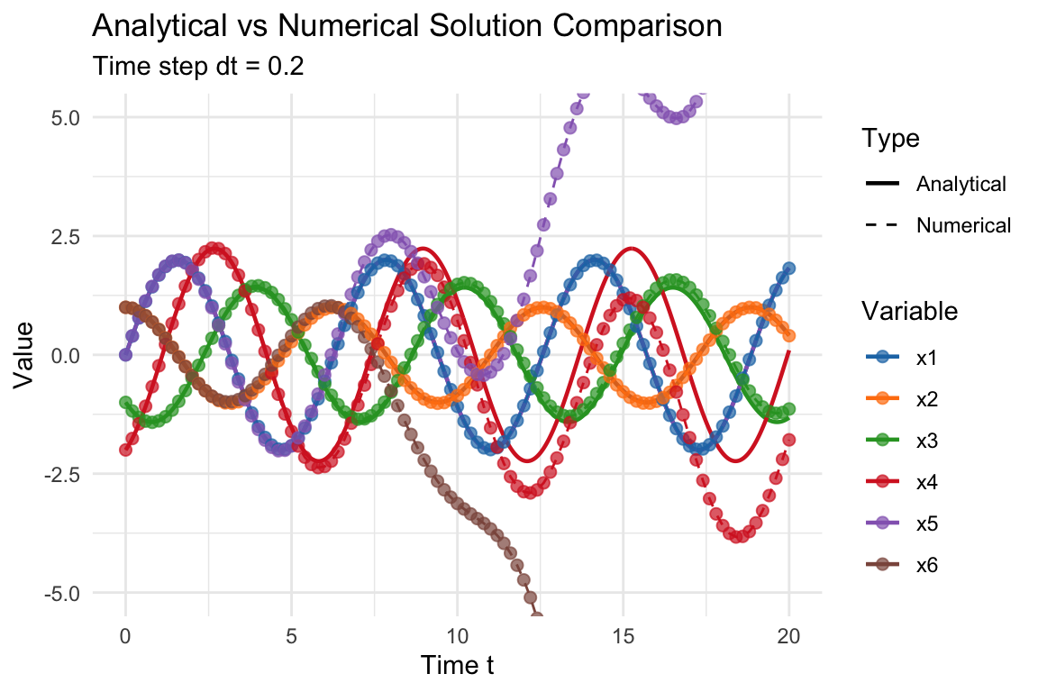
Numerical solution witb \Delta t = 0.2. Notice the drift for components x_6 and x_5.
Dummy-Variable Reduction
Variable Classification
- Differential variables: x_1, x_2, x_3, x_4. x_5
- Algebraic variables: x_6
We attempt to solve for u_6 and v_{\text{dot}}, but due to the presence of \lambda, the system is not yet solvable explicitly. We proceed by differentiating.
Step 1: Differentiate Constraints
Differentiate \text{(Constraint 1)} = \cos t-x_6:
\frac{\mathrm{d}\text{(Constraint 1)} }{\mathrm{d}t} = -\sin t - x'_6
Substitute known differential variables:
\color{DarkRed}\text{(Constraint 2)} = x_5 - 2\sin t
x'_1 not found, continue index reduction.
Step 2: Differentiate Constraints
Differentiate \text{(Constraint 2)}
\frac{\mathrm{d}\text{(Constraint 2)} }{\mathrm{d}t} = x'_5 - 2\cos t \quad\implies\quad \color{DarkRed}\text{(Constraint 3)} = \sin t - 2\cos t - x_4
x'_1 not found, continue index reduction.
Step 3: Differentiate Constraints
Differentiate \text{(Constraint 3)}:
\frac{\mathrm{d}\text{(Constraint 3)} }{\mathrm{d}t} = \cos t + 2\sin t - x'_4 \quad\implies\quad \color{DarkRed}\text{(Constraint 4)} = \cos t + \sin t + x_3
x'_1 not found, continue index reduction.
Step 4: Differentiate Constraints
Differentiate \text{(Constraint 4)}:
\frac{\mathrm{d}\text{(Constraint 4)}}{\mathrm{d}t} = -\sin t + \cos t + x'_3 \quad\implies\quad \color{DarkRed}\text{(Constraint 5)} = \cos t - x_2
x'_1 not found, continue index reduction.
Step 5: Differentiate Constraints
Differentiate \text{(Constraint 5)}:
\frac{\mathrm{d}\text{(Constraint 5)}}{\mathrm{d}t} = -\sin t - x'_2 \quad\implies\quad \color{DarkRed}\text{(Constraint 6)} = -2\sin t + x_1
x'_1 not found, continue index reduction.
Step 6: Differentiate Constraints
Differentiate \text{(Constraint 6)}:
\frac{\mathrm{d}\text{(Constraint 6)}}{\mathrm{d}t} = -2\cos t - 2\sin t + x'_1
x'_1 found, index reduction complete
\left\{ \begin{aligned} \color{blue} x_6' &\color{blue}= \sin t - x_5 \\ \color{blue} x_5' &\color{blue}= \sin t - x_4 \\ \color{blue} x_4' &\color{blue}= \sin t - x_3 \\ \color{blue} x_3' &\color{blue}= \sin t - x_2 \\ \color{blue} x_2' &\color{blue}= \sin t - x_1 \\ \color{blue} x_1' &\color{blue}= 2\sin t \end{aligned} \right. \qquad \left\{ \begin{aligned} \color{DarkRed}\text{(Constraint 1)} &\color{DarkRed} = \cos t - x_6 = 0\\ \color{DarkRed}\text{(Constraint 2)} &\color{DarkRed} = x_5 - 2\sin t = 0\\ \color{DarkRed}\text{(Constraint 3)} &\color{DarkRed} = \sin t - 2 \cos t - x_4 = 0\\ \color{DarkRed}\text{(Constraint 4)} &\color{DarkRed} = \sin t + \cos t + x_3 = 0\\ \color{DarkRed}\text{(Constraint 5)} &\color{DarkRed} = \cos t - x_2 = 0\\ \color{DarkRed}\text{(Constraint 6)} &\color{DarkRed} = x_1 -2\sin t = 0 \end{aligned} \right.
Applied 6 time differentiation, the index is 6.
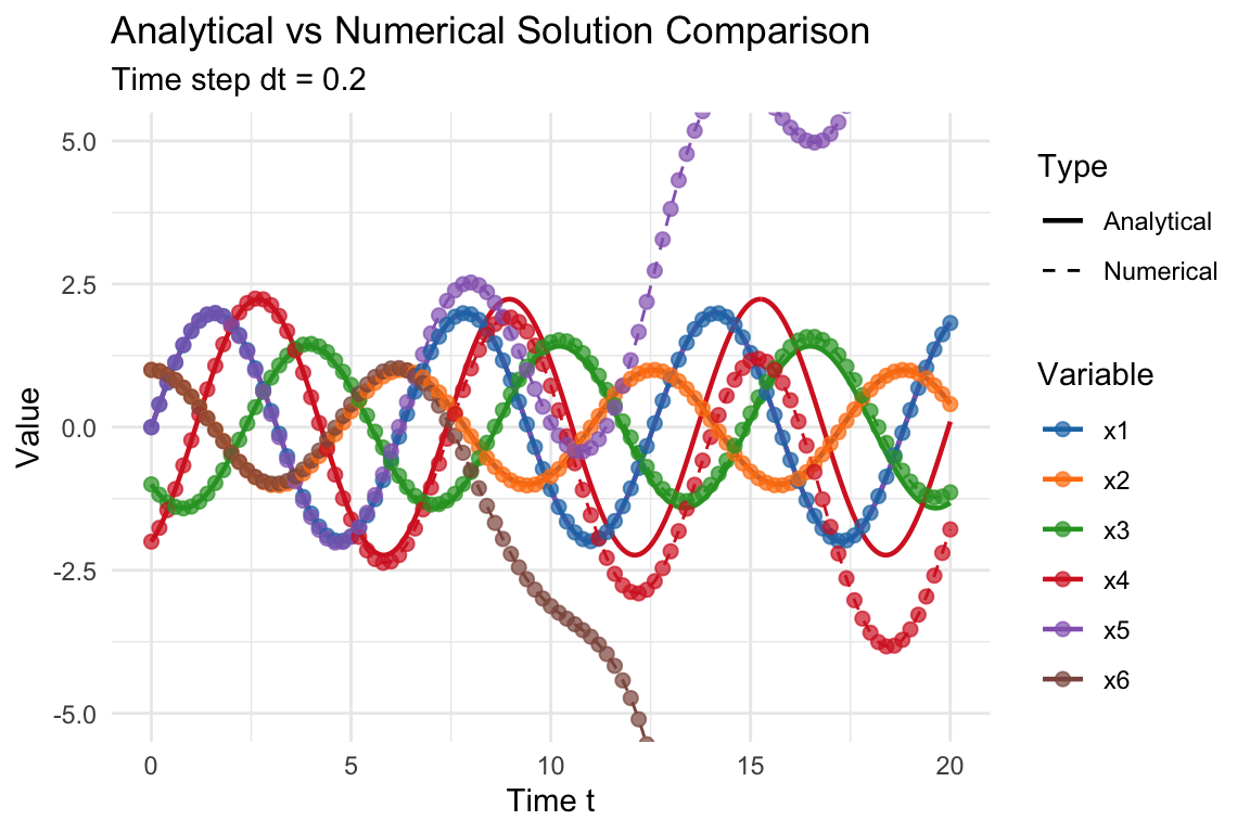
Numerical solution witb \Delta t = 0.2. Notice the drift for components x_6 and x_5.