1 Optimization Algorithms

Author

Affiliation

Enrico Bertolazzi

University of Trento, Department of Industrial Engineering

This chapter turns the optimality conditions of the course notes into algorithms. The first section treats smooth unconstrained minimization and supplies the globalization and quasi-Newton tools reused in the second, which develops methods for constrained nonlinear programming.

1.1 Unconstrained Optimization

Consider the smooth optimization problem

\min_{\bm x\in\mathbb R^n} f(\bm x). \tag{1.1}

The optimality conditions developed earlier in this part describe a solution. This section addresses the complementary computational question: how should an iterate be moved toward a stationary point, and how can one decide whether the computed result is trustworthy?

The presentation separates three ingredients that every practical method must specify:

a local model of the objective;
a step computation based on that model;
a globalization and stopping strategy.

After this section, the downloadable unconstrained-minimization laboratory can be used to compare these choices on classical test problems.

Learning objectives

After studying this section, the reader should be able to

distinguish local convergence from convergence from a remote initial point;
explain how conditioning affects gradient and Newton iterations;
apply Armijo and Wolfe line searches;
construct modified-Newton and BFGS directions;
explain the acceptance test of a trust-region method;
interpret termination tests and common solver failure modes.

Throughout this section, the analytical gradient \nabla f(\bm x) remains a row vector, as established in the mathematical preliminaries. For numerical linear algebra we use the column vector

\bm q(\bm x):=\nabla f(\bm x)^T, \qquad \bm H(\bm x):=\nabla^2f(\bm x).

From optimality conditions to an iteration

If f is differentiable and \bm x^\star is an unconstrained local minimizer, then

\bm q(\bm x^\star)=\bm0.

If f is twice differentiable, a necessary second-order condition is \bm H(\bm x^\star)\succeq\bm0. The sufficient condition \bm H(\bm x^\star)\succ\bm0 implies a strict local minimum and local quadratic growth.

These facts suggest solving the nonlinear system \bm q(\bm x)=\bm0. Optimization algorithms exploit more structure than a generic root solver: they also seek a reduction of f and can use negative curvature to escape points that are not minima.

Most smooth methods have the form

\bm x_{k+1}=\bm x_k+\alpha_k\bm p_k, \tag{1.2}

where \bm p_k is a search direction and \alpha_k>0 is a step length. A direction is a descent direction when

\bm q_k^T\bm p_k<0. \tag{1.3}

Indeed, differentiability gives

f(\bm x_k+\alpha\bm p_k) =f(\bm x_k)+\alpha\bm q_k^T\bm p_k+o(\alpha),

so every sufficiently small positive step decreases the objective. This is a local statement; it does not say that a full step \alpha=1 is safe.

Conditioning and scaling

The quadratic function

f(\bm x)=\frac12\bm x^T\bm A\bm x-\bm b^T\bm x, \qquad \bm A\succ\bm0, \tag{1.4}

is the basic model for understanding conditioning. Its minimizer solves \bm A\bm x^\star=\bm b. Let

0<\lambda_{\min}\leq\lambda_{\max}

be the extreme eigenvalues of \bm A. The spectral condition number is

\kappa_2(\bm A)=\frac{\lambda_{\max}}{\lambda_{\min}}.

For steepest descent with an exact line search, the error in the \bm A-norm satisfies

\frac{\|\bm x_{k+1}-\bm x^\star\|_{\bm A}} {\|\bm x_k-\bm x^\star\|_{\bm A}} \leq \frac{\kappa_2(\bm A)-1}{\kappa_2(\bm A)+1}. \tag{1.5}

When \kappa_2(\bm A) is large, the factor is close to one and the iterates zigzag across a narrow valley. Poor conditioning is therefore not merely a linear-algebra issue: it directly controls algorithmic progress.

Variable scaling replaces \bm x=\bm D\bm z and minimizes \widehat f(\bm z)=f(\bm D\bm z). A good diagonal scaling makes typical components of \bm z and the curvature along coordinate directions comparable. It also makes step and gradient tolerances more meaningful.

Scaling is part of the model

Multiplying the objective by a constant does not change its minimizer, but it does change raw function and gradient magnitudes. Similarly, changing the units of one variable changes the apparent conditioning. Solver tolerances must therefore be interpreted together with the scaling of the model.

Convergence rates

Let e_k=\|\bm x_k-\bm x^\star\|. The sequence converges with order p\geq1 if, asymptotically,

e_{k+1}\leq C e_k^p \tag{1.6}

for some constant C>0. The main cases are:

Rate	Characterization	Typical method near a regular minimizer
Linear	e_{k+1}\leq\rho e_k, 0<\rho<1	gradient method
Superlinear	e_{k+1}/e_k\to0	BFGS with suitable line search
Quadratic	e_{k+1}\leq C e_k^2	exact Newton method

These are local rates. They describe behavior after the iterates enter a neighborhood in which the model is accurate. They do not guarantee that a method started far from \bm x^\star will reach that neighborhood.

A global convergence theorem normally states that every accumulation point is stationary, or that \|\bm q_k\|\to0, under specified assumptions. It does not mean convergence to a global minimizer of a nonconvex function.

Gradient methods

The steepest-descent direction in the Euclidean norm is

\bm p_k=-\bm q_k.

If the gradient is L-Lipschitz continuous, the descent lemma gives

f(\bm x_k-\alpha\bm q_k) \leq f(\bm x_k) -\alpha\left(1-\frac{L\alpha}{2}\right)\|\bm q_k\|^2.

Thus every fixed step 0<\alpha<2/L decreases the objective unless \bm q_k=\bm0. The estimate is useful theoretically, but L is rarely known accurately. A line search estimates an acceptable scale from function values.

Gradient descent is inexpensive and robust but uses no curvature information. It is useful for large problems and as a safeguard, although it can be very slow on badly conditioned objectives.

Line-search globalization

Given a descent direction \bm p_k, a line search considers

\phi_k(\alpha)=f(\bm x_k+\alpha\bm p_k).

Exact minimization of \phi_k is normally unnecessary. Practical methods seek a step that is inexpensive to compute and sufficiently productive.

Armijo sufficient decrease

The Armijo condition is

f(\bm x_k+\alpha\bm p_k) \leq f(\bm x_k)+c_1\alpha\bm q_k^T\bm p_k, \qquad 0<c_1<1. \tag{1.7}

Since \bm q_k^T\bm p_k<0, the right-hand side is smaller than f(\bm x_k). Backtracking begins with \alpha=1 and repeatedly replaces \alpha by \beta\alpha, with 0<\beta<1, until Equation 1.7 holds. Common choices are c_1=10^{-4} and \beta\in[0.1,0.8] [@armijo1966minimization].

Armijo decrease prevents steps that are too long, but by itself it can accept steps that are unnecessarily short.

Wolfe curvature conditions

The Wolfe conditions add

\bm q(\bm x_k+\alpha\bm p_k)^T\bm p_k \geq c_2\bm q_k^T\bm p_k, \qquad c_1<c_2<1. \tag{1.8}

The strong Wolfe condition instead requires

\left| \bm q(\bm x_k+\alpha\bm p_k)^T\bm p_k \right| \leq c_2|\bm q_k^T\bm p_k|. \tag{1.9}

The curvature test ensures that the directional derivative has changed sufficiently. It is especially important for quasi-Newton methods because it helps preserve positive curvature in the BFGS update.

Backtracking line search

Choose a descent direction \bm p_k and set \alpha\leftarrow1.
While the Armijo condition fails, set \alpha\leftarrow\beta\alpha.
Accept \bm x_{k+1}=\bm x_k+\alpha\bm p_k.

The full step should be tested first. Near a regular minimizer, Newton and BFGS methods need to recover \alpha=1 in order to exhibit their fast local rates.

Newton and modified-Newton methods

At \bm x_k, the quadratic Taylor model is

m_k(\bm p) =f(\bm x_k)+\bm q_k^T\bm p +\frac12\bm p^T\bm H_k\bm p. \tag{1.10}

If \bm H_k is nonsingular, stationarity of the model gives

\bm H_k\bm p_k=-\bm q_k. \tag{1.11}

Near a minimizer at which \bm H(\bm x^\star)\succ\bm0, the full Newton step is well defined and converges quadratically, provided the Hessian is sufficiently regular. Far from the solution, however, the Hessian can be indefinite and the Newton direction need not be a descent direction.

A modified-Newton method replaces \bm H_k with a positive-definite matrix

\bm B_k=\bm H_k+\tau_k\bm I, \qquad \tau_k\geq0, \tag{1.12}

and solves \bm B_k\bm p_k=-\bm q_k. The shift can be increased until a Cholesky factorization succeeds. Then

\bm q_k^T\bm p_k =-\bm p_k^T\bm B_k\bm p_k<0

for every nonzero step. This is a modified-Newton or Levenberg–Marquardt-type regularization [@marquardt1963algorithm]. A line search supplies globalization; close to a well-conditioned minimizer the shift should return to zero.

BFGS and limited-memory methods

Quasi-Newton methods replace the exact Hessian by an approximation. Define

\bm s_k=\bm x_{k+1}-\bm x_k, \qquad \bm y_k=\bm q_{k+1}-\bm q_k.

The secant equation

\bm B_{k+1}\bm s_k=\bm y_k \tag{1.13}

requires the new matrix to reproduce the observed change of gradient. The BFGS update is

\bm B_{k+1} =\bm B_k -\frac{\bm B_k\bm s_k\bm s_k^T\bm B_k} {\bm s_k^T\bm B_k\bm s_k} +\frac{\bm y_k\bm y_k^T}{\bm y_k^T\bm s_k}. \tag{1.14}

If \bm B_k\succ\bm0 and \bm y_k^T\bm s_k>0, then \bm B_{k+1}\succ\bm0. A Wolfe line search normally enforces this curvature condition. The search direction is obtained from

\bm B_k\bm p_k=-\bm q_k.

BFGS avoids exact second derivatives and generally achieves superlinear local convergence. Limited-memory BFGS stores only a small number of recent pairs (\bm s_k,\bm y_k), making it suitable for large problems. Its lower memory cost comes at the price of a less complete curvature model.

Trust-region globalization

A trust-region method computes the step by approximately solving \min_{\|\bm p\|\leq\Delta_k} m_k(\bm p) =f_k+\bm q_k^T\bm p+\frac12\bm p^T\bm B_k\bm p. \tag{1.15}

The radius \Delta_k defines the region in which the local model is trusted. After computing a trial step, the agreement between model and objective is measured by

\rho_k =\frac{f(\bm x_k)-f(\bm x_k+\bm p_k)} {m_k(\bm0)-m_k(\bm p_k)}. \tag{1.16}

If \rho_k is small or negative, the model is poor: reject the step and reduce \Delta_k.
If \rho_k is moderate, accept the step and keep a comparable radius.
If \rho_k is close to one and the step reaches the boundary, accept it and enlarge \Delta_k.

Unlike a line search, a trust region does not commit to a direction before choosing the step size. It can exploit directions of negative curvature and is therefore particularly effective for indefinite Hessians. Dogleg methods are convenient for positive-definite models; truncated conjugate gradients are attractive for large systems and can stop when negative curvature is detected.

Stopping tests and diagnostic evidence

No single floating-point test proves that an iterate is a minimizer. A robust implementation records several diagnostics.

First-order stationarity

A scaled gradient test can be written as

\|\bm q_k\|_\infty \leq \varepsilon_a+\varepsilon_r\|\bm q_0\|_\infty. \tag{1.17}

The scaling should be chosen consistently with the units of the variables. Comparing \|\bm q_k\| directly with 1+|f_k| is dimensionally questionable because the gradient scales as objective divided by variable.

Step and objective changes

Small values of

\frac{\|\bm x_{k+1}-\bm x_k\|} {1+\|\bm x_k\|} \quad\text{and}\quad \frac{|f_{k+1}-f_k|}{1+|f_k|}

are useful secondary tests. They are not sufficient by themselves: a line search can produce a tiny step because the direction is poor, and a flat or badly scaled objective can change very little far from stationarity.

Second-order evidence

At a reported solution, inspect the smallest eigenvalue of the Hessian when this is computationally feasible. A small gradient with a negative Hessian eigenvalue indicates a saddle point, not a local minimum. Near-zero eigenvalues indicate degeneracy and make the observed convergence rate sensitive to roundoff and scaling.

Derivative verification

Before diagnosing an algorithm, verify the derivatives. For a normalized direction \bm d, compare

\nabla f(\bm x)\bm d \quad\text{with}\quad \frac{f(\bm x+h\bm d)-f(\bm x-h\bm d)}{2h}.

The discrepancy should initially decrease like h^2 and then increase when roundoff dominates. Testing several random directions is more informative than checking coordinate directions alone.

A solver status is not a certificate

A success flag, a small step, agreement between two solvers, or a small gradient taken separately is not conclusive. The interpretation should combine stationarity, curvature, scaling, iteration history, and sensitivity to the initial point.

Choosing a method

Situation	Suitable first choice	Main diagnostic
Small smooth problem, accurate Hessian	damped or trust-region Newton	Hessian definiteness and full-step recovery
Smooth problem, Hessian expensive	BFGS	curvature pairs and gradient norm
Large smooth problem	limited-memory BFGS	projected/scaled gradient and line-search history
Hessian-vector products available	Newton–CG	residual and negative-curvature detection
Strong nonconvexity	trust-region Newton	ratio of actual to predicted reduction
Poorly scaled variables	rescale before selecting the method	componentwise steps and gradients

The method should match the information available. Supplying an inaccurate Hessian to Newton’s method can be worse than using a carefully safeguarded quasi-Newton approximation.

Computational laboratory

The notebook 01 – Unconstrained minimization implements gradient, Newton, modified-Newton, BFGS, and SciPy methods. It records iteration histories and examines Rosenbrock, Himmelblau, Beale, Powell singular, Brown badly scaled, and Freudenstein–Roth problems. Its purpose is to test the theory above rather than to replace it.

Download: unconstrained-minimization algorithms and diagnostic experiments

Exercises

The labels indicate the intended level: F fundamental, C computational, and A advanced. Each item includes a short starting hint.

F. For the quadratic problem Equation 1.4, derive the exact line-search step for the steepest-descent direction. Hint: minimize the one-variable quadratic f(\bm x_k+\alpha\bm p_k).
F. Show that a positive-definite modified-Newton matrix produces a descent direction whenever \bm q_k\neq\bm0. Hint: premultiply the Newton equation by the direction transpose.
F. Explain why Armijo backtracking alone does not guarantee \bm y_k^T\bm s_k>0 for a BFGS update. Hint: compare Armijo with the curvature Wolfe condition.
C. Apply one BFGS update to a two-dimensional quadratic and verify the secant equation Equation 1.13. Hint: compute the matrix-vector product after the update, not only the updated entries.
A. For an indefinite quadratic model, compare the Newton step with the solution of Equation 1.15. Hint: inspect the most negative curvature direction.
A. Construct an example in which a relative objective-change test terminates far from a stationary point. Hint: rescale or offset the objective while leaving its gradient appreciable.
C. Use directional finite differences to determine an appropriate range of h for derivative checking in double precision. Hint: plot the error against h on logarithmic axes.
C. In the computational laboratory, compare the convergence history from two distinct attraction basins of the Himmelblau function. Hint: retain the complete iteration history and not only the final point.

1.2 Constrained Optimization

The optimality conditions developed in the preceding sections characterize candidate minimizers. This section turns the constrained conditions into numerical algorithms, building on the local models, line searches, quasi-Newton updates, and trust-region ideas developed in Section 1.1. The presentation follows the standard globalization framework of @nocedal2006numerical, @bertsekas2016nonlinear, and @fletcher2000practical.

Throughout this section, gradients used in linear algebra formulas are column vectors. Thus, if the analytical convention established in the mathematical preliminaries writes \nabla f(\bm x) as a row vector, here

\bm q(\bm x)=\nabla f(\bm x)^T.

The symbol \bm g is reserved for inequality constraints, whereas \bm q always denotes the objective gradient. Throughout, n is the number of variables, m_h the number of equality constraints, and m_g the number of inequality constraints; \bm J_h and \bm J_g are the corresponding Jacobians.

The NLP viewpoint and algorithmic map

A smooth nonlinear programming problem (NLP) can be written in the form

\begin{aligned} \min_{\bm x\in\mathbb R^n}\quad & f(\bm x),\\ \text{subject to}\quad &\bm h(\bm x)=\bm0,\\ &\bm g(\bm x)\geq\bm0,\\ &\bm\ell\leq\bm x\leq\bm u. \end{aligned} \tag{1.18}

The numerical methods in this section should not be viewed as unrelated algorithms. Most modern smooth NLP methods are different ways of solving, regularizing, or approximating the KKT equations. They differ mainly in four choices:

how feasibility is enforced or approached;
how complementarity for inequalities is handled;
how the Lagrangian Hessian is represented;
how the local Newton model is globalized away from the solution.

This viewpoint leads to the following map.

Family	Treatment of constraints	Local model	Typical globalization
Projected methods	explicit projection	gradient/Newton	line search
Penalty methods	penalize violation	unconstrained	penalty continuation
Augmented Lagrangian	multipliers + finite penalty	unconstrained/bound constrained	outer multiplier/penalty update
Active-set SQP	predict active inequalities	QP	merit/filter line search or trust region
Interior-point	perturbed complementarity	primal-dual KKT system	barrier continuation + filter/line search
Sequential convex methods	convex local approximation	LP/QP/convex program	trust region/filter

The common computational core is frequently a saddle-point system

\begin{bmatrix} \bm B & \bm A^T\\ \bm A & \bm0 \end{bmatrix} \begin{bmatrix} \bm p\\ \bm y \end{bmatrix} = \begin{bmatrix} \bm r_1\\ \bm r_2 \end{bmatrix}, \tag{1.19}

possibly after elimination of slack variables. Understanding this structure is therefore more important than memorizing individual solver names.

Local models and globalization

A constrained Newton model is reliable only locally. A practical NLP method therefore has two layers:

a local model, usually Newton, quasi-Newton, QP, or a primal-dual Newton system;
a globalization mechanism, usually a merit-function line search, a filter, a trust region, or a continuation parameter.

Near a regular solution the globalization should become inactive so that the fast local convergence of the underlying Newton-type iteration is recovered.

Unconstrained methods as the local computational model

The unconstrained algorithms developed in Section 1.1 provide the local computational engine for many constrained methods below. Penalty and augmented-Lagrangian approaches repeatedly solve unconstrained subproblems, while SQP and interior-point methods reuse Newton, quasi-Newton, line-search, and trust-region principles on constrained local models. ### Simple constraints: projection and bound constraints

When the feasible set \Omega is simple enough that the Euclidean projection

P_\Omega(\bm z) =\operatorname*{argmin}_{\bm x\in\Omega}\frac12\|\bm x-\bm z\|^2

is inexpensive, a projected-gradient iteration is

\bm x_{k+1} =P_\Omega\!\left(\bm x_k-\alpha_k\bm q_k\right). \tag{1.20}

For box constraints, projection is componentwise,

[P_\Omega(\bm z)]_i =\min\{u_i,\max\{\ell_i,z_i\}\}.

The natural first-order residual is the gradient mapping

\bm G_\alpha(\bm x) =\frac{1}{\alpha} \left[\bm x-P_\Omega(\bm x-\alpha\bm q(\bm x))\right].

Thus \bm G_\alpha(\bm x)=\bm0 characterizes first-order stationarity for a closed convex feasible set. Projected Newton and active-set bound-constrained methods replace the gradient step by a second-order step on the currently free variables.

Penalty methods and exact penalties

A quadratic exterior penalty for equality constraints is

P_\rho(\bm x) =f(\bm x)+\frac{\rho}{2}\|\bm h(\bm x)\|_2^2. \tag{1.21}

For inequalities \bm g(\bm x)\geq\bm0, one may add

\frac{\rho}{2}\|\min\{\bm g(\bm x),\bm0\}\|_2^2.

If the inner minimizations are sufficiently accurate and \rho\to\infty, limit points can approach constrained solutions under standard regularity assumptions. The drawback is visible from the Hessian: near feasibility it contains the term

\rho\bm J_h^T\bm J_h,

so increasing \rho can make the subproblem severely ill-conditioned.

An important alternative is the nonsmooth exact \ell_1 penalty

P_\rho^{(1)}(\bm x) =f(\bm x) +\rho\|\bm h(\bm x)\|_1 +\rho\|\min\{\bm g(\bm x),\bm0\}\|_1. \tag{1.22}

Under suitable constraint qualifications, a finite sufficiently large \rho is enough for a local constrained minimizer to be a local minimizer of the penalty function. This exactness explains why \ell_1 functions are also useful as merit functions in SQP methods.

The multiplier hidden in the quadratic penalty

The quadratic penalty is not merely a crude device: it already contains a multiplier estimate, and seeing it explains the augmented Lagrangian of Section 1.2.7. Stationarity of Equation 1.21 gives

\bm q(\bm x_\rho)+\rho\bm J_h(\bm x_\rho)^T\bm h(\bm x_\rho)=\bm0, \qquad\text{that is}\qquad \bm q(\bm x_\rho)=\bm J_h(\bm x_\rho)^T\bigl(-\rho\bm h(\bm x_\rho)\bigr).

Comparing with the stationarity condition \bm q=\bm J_h^T\bm\lambda of the constrained problem shows that

\boxed{\;\bm\lambda\approx-\rho\,\bm h(\bm x_\rho).\;} \tag{1.23}

The multiplier is recovered only in the limit, because it is obtained by multiplying a quantity that tends to zero by one that tends to infinity: this product is exactly the source of the ill-conditioning. The augmented Lagrangian removes the difficulty by carrying \bm\lambda as an explicit variable and using Equation 1.23 only as a correction to the current estimate, which keeps \rho finite.

Equality-constrained minimization

Consider

\begin{aligned} \min_{\bm x\in\mathbb R^n}\quad & f(\bm x),\\ \text{subject to}\quad & \bm h(\bm x)=\bm0, \end{aligned}

with \bm h:\mathbb R^n\to\mathbb R^{m_h}. Consistently with the preceding KKT chapter, define

\mathcal L(\bm x,\bm\lambda) =f(\bm x)-\bm\lambda^T\bm h(\bm x),

and let \bm J(\bm x) be the Jacobian of \bm h. The first-order system is

\bm F(\bm x,\bm\lambda) = \begin{bmatrix} \nabla_x\mathcal L(\bm x,\bm\lambda)^T\\ \bm h(\bm x) \end{bmatrix} =\bm0. \tag{1.24}

Newton’s method for the KKT system

The Jacobian of Equation 1.24, written out in full in Equation 1.26 below, has lower-left block \bm J_k and upper-right block -\bm J_k^T. For numerical factorization it is useful to multiply the feasibility equation by -1. This row scaling does not change the Newton step and gives the symmetric-indefinite system

\begin{bmatrix} \bm W_k & -\bm J_k^T\\ -\bm J_k & \bm0 \end{bmatrix} \begin{bmatrix} \bm p_k\\ \delta\bm\lambda_k \end{bmatrix} = \begin{bmatrix} -\nabla_x\mathcal L_k^T\\ \bm h_k \end{bmatrix}, \tag{1.25}

where

\bm W_k=\nabla_{xx}^2\mathcal L(\bm x_k,\bm\lambda_k).

The second block row is still the linearized feasibility equation \bm J_k\bm p_k=-\bm h_k. The coefficient matrix is symmetric but indefinite; a Cholesky factorization of the complete KKT matrix is therefore not appropriate. Without the row scaling, the raw Newton Jacobian Equation 1.26 is algebraically equivalent but nonsymmetric.

If LICQ holds and the reduced Hessian is positive definite, the KKT matrix is nonsingular near the solution. The full Newton step is then locally quadratically convergent.

SQP as Newton’s method applied to the KKT equations

The relation between Newton’s method and SQP is exact, not merely heuristic. For the equality-constrained problem define the primal–dual variable

\bm z= \begin{bmatrix} \bm x\\ \bm\lambda \end{bmatrix}, \qquad \bm F(\bm z)= \begin{bmatrix} \bm q(\bm x)-\bm J(\bm x)^T\bm\lambda\\ \bm h(\bm x) \end{bmatrix}.

A KKT point is a zero of \bm F. Its Jacobian is

\bm F'(\bm z)= \begin{bmatrix} \nabla_{xx}^2\mathcal L(\bm x,\bm\lambda) & -\bm J(\bm x)^T\\ \bm J(\bm x) & \bm0 \end{bmatrix}. \tag{1.26}

Newton’s method for \bm F(\bm z)=\bm0 computes \Delta\bm z_k=(\bm p_k,\delta\bm\lambda_k) from

\bm F'(\bm z_k)\Delta\bm z_k=-\bm F(\bm z_k).

Writing the first block row explicitly gives

\bm W_k\bm p_k-\bm J_k^T\delta\bm\lambda_k =-\bm q_k+\bm J_k^T\bm\lambda_k,

or, after defining the new multiplier estimate

\widehat{\bm\lambda}_{k+1} =\bm\lambda_k+\delta\bm\lambda_k,

\bm W_k\bm p_k-\bm J_k^T\widehat{\bm\lambda}_{k+1} =-\bm q_k. \tag{1.27}

The second block row is

\bm J_k\bm p_k=-\bm h_k. \tag{1.28}

Now consider the quadratic program

\begin{aligned} \min_{\bm p}\quad & q_k(\bm p) =\bm q_k^T\bm p+\frac12\bm p^T\bm W_k\bm p,\\ \text{subject to}\quad & \bm h_k+\bm J_k\bm p=\bm0. \end{aligned} \tag{1.29}

Its Lagrangian is

\mathcal L_k^{\rm QP}(\bm p,\widehat{\bm\lambda}) = \bm q_k^T\bm p+ \frac12\bm p^T\bm W_k\bm p - \widehat{\bm\lambda}^T (\bm h_k+\bm J_k\bm p).

The QP KKT equations are precisely Equation 1.27 and Equation 1.28. Multiplying the latter by -1 produces the symmetric system Equation 1.25. Consequently,

\boxed{\text{exact-Hessian SQP step} \equiv \text{Newton step for the nonlinear KKT equations}.}

The distinction is conceptual rather than algebraic. Newton views the problem as a nonlinear system in (\bm x,\bm\lambda); SQP views the same equations as the optimality conditions of a local quadratic optimization problem. The SQP viewpoint is particularly valuable because inequalities and bounds can be retained explicitly in the QP subproblem.

Why the Lagrangian Hessian appears

It is important not to replace \bm W_k blindly by \nabla^2 f(\bm x_k). Differentiating stationarity gives

\bm W_k = \nabla^2 f(\bm x_k) - \sum_{i=1}^{m_h} \lambda_{k,i}\nabla^2 h_i(\bm x_k).

Thus the curvature of the constraint manifold contributes to the Newton model. Omitting these terms generally destroys exact Newton equivalence and can reduce the local convergence rate.

Nonsingularity of the KKT Jacobian

Let \bm z^\star=(\bm x^\star,\bm\lambda^\star) be a KKT point. Suppose \bm J_\star has full row rank (LICQ), and let the columns of \bm Z_\star form a basis for the tangent space

\mathcal T_\star=\ker(\bm J_\star).

Assume the second-order sufficient condition

\bm d^T\bm W_\star\bm d>0 \qquad \text{for every }\bm d\neq\bm0 \text{ with }\bm J_\star\bm d=\bm0, \tag{1.30}

or equivalently

\bm Z_\star^T\bm W_\star\bm Z_\star\succ\bm0.

Then the KKT Jacobian is nonsingular. Indeed, if

\begin{bmatrix} \bm W_\star&-\bm J_\star^T\\ \bm J_\star&\bm0 \end{bmatrix} \begin{bmatrix}\bm d\\\bm v\end{bmatrix} =\bm0,

then \bm J_\star\bm d=\bm0. Multiplying the first row by \bm d^T gives \bm d^T\bm W_\star\bm d=0, because \bm d^T\bm J_\star^T\bm v=0. By Equation 1.30, \bm d=\bm0. The first row then gives \bm J_\star^T\bm v=\bm0, and full row rank of \bm J_\star implies \bm v=\bm0.

Local quadratic convergence of exact-Hessian SQP

The preceding equivalence permits the standard Newton convergence theorem to be applied directly.

Theorem 1.1 (Local quadratic convergence of SQP) Suppose that f and \bm h are sufficiently smooth in a neighborhood of a KKT point (\bm x^\star,\bm\lambda^\star), LICQ holds there, the second-order sufficient condition Equation 1.30 holds, and \bm F' is locally Lipschitz continuous. Then there exists a neighborhood \mathcal N of (\bm x^\star,\bm\lambda^\star) such that, for every (\bm x_0,\bm\lambda_0)\in\mathcal N, exact-Hessian SQP with full steps is well defined and

\left\| \begin{bmatrix} \bm x_{k+1}-\bm x^\star\\ \bm\lambda_{k+1}-\bm\lambda^\star \end{bmatrix} \right\| \leq C \left\| \begin{bmatrix} \bm x_k-\bm x^\star\\ \bm\lambda_k-\bm\lambda^\star \end{bmatrix} \right\|^2 \tag{1.31}

for every k\ge0 and some constant C>0.

To see the mechanism, write

\bm e_k=\bm z_k-\bm z^\star.

Newton’s update is

\bm e_{k+1} = \bm e_k-\bm F'(\bm z_k)^{-1}\bm F(\bm z_k).

Since \bm F(\bm z^\star)=\bm0,

\bm F(\bm z_k) = \int_0^1 \bm F'(\bm z^\star+t\bm e_k)\bm e_k\,dt.

Hence

\bm e_{k+1} = \bm F'(\bm z_k)^{-1} \int_0^1 \left[ \bm F'(\bm z_k)- \bm F'(\bm z^\star+t\bm e_k) \right] \bm e_k\,dt.

Local nonsingularity makes \|\bm F'(\bm z_k)^{-1}\| uniformly bounded, and Lipschitz continuity gives

\left\| \bm F'(\bm z_k)- \bm F'(\bm z^\star+t\bm e_k) \right\| \leq L(1-t)\|\bm e_k\|.

Integration therefore yields

\|\bm e_{k+1}\| \leq \frac{ML}{2}\|\bm e_k\|^2,

which proves Equation 1.31.

For inequality-constrained NLP, once the correct active set has been identified, the locally active inequalities can be appended to \bm h(\bm x)=\bm0. Under LICQ, a suitable second-order sufficient condition, and nondegeneracy such as strict complementarity, the same Newton argument applies to this active KKT system. This is the source of the local quadratic rate of exact-Hessian active-set SQP.

Quasi-Newton SQP and superlinear convergence

In practice \bm W_k is often replaced by \bm B_k. The SQP equations are then an inexact or quasi-Newton approximation to the KKT Newton equations. Quadratic convergence is generally lost, but superlinear convergence is possible if the Hessian approximation becomes sufficiently accurate along the computed steps. A constrained analogue of the Dennis–Moré condition is, schematically,

\frac{\|(\bm B_k-\bm W_\star)\bm p_k\|} {\|\bm p_k\|} \longrightarrow0,

with the relevant condition often required only on the tangent space; in the unconstrained case this is exactly the characterization of @dennis1974characterization. BFGS updates of the Lagrangian Hessian are designed to achieve this behavior while avoiding second derivatives.

Sequential quadratic programming

Replacing \bm W_k by a symmetric approximation \bm B_k produces the equality-constrained SQP subproblem

\begin{aligned} \min_{\bm p}\quad & \bm q_k^T\bm p+\frac12\bm p^T\bm B_k\bm p,\\ \text{subject to}\quad & \bm h_k+\bm J_k\bm p=\bm0. \end{aligned} \tag{1.32}

Its KKT equations have the same block structure as Equation 1.25. Hence Newton on the nonlinear KKT equations and SQP with the exact Lagrangian Hessian produce the same local step.

A line search can be based on the exact \ell_1 merit function

\phi_\rho(\bm x)=f(\bm x)+\rho\|\bm h(\bm x)\|_1, \tag{1.33}

where \rho must be large enough to balance objective reduction and feasibility improvement.

Algorithm 2: Damped Newton–SQP for equality constraints

Input: \bm x_0, \bm\lambda_0, dual and primal tolerances \varepsilon_d, \varepsilon_p.

Output: An approximate KKT pair (\bm x,\bm\lambda).

Set (\bm x,\bm\lambda)\leftarrow(\bm x_0,\bm\lambda_0).
Repeat:
1. Evaluate \bm h, \bm J and \bm r_d=\nabla f(\bm x)^T-\bm J^T\bm\lambda.
2. If \|\bm r_d\|\leq\varepsilon_d and \|\bm h\|\leq\varepsilon_p, return (\bm x,\bm\lambda).
3. Form a stabilized or BFGS approximation \bm B of \nabla_{xx}^2\mathcal L.
4. Solve the KKT system Equation 1.25 for (\bm p,\delta\bm\lambda), replacing \bm W by \bm B.
5. Choose the merit parameter \rho.
6. Choose \alpha\in(0,1] with a merit-function or filter line search.
7. Set \bm x\leftarrow\bm x+\alpha\bm p and \bm\lambda\leftarrow\bm\lambda+\alpha\delta\bm\lambda.
Until the maximum number of iterations is reached.

For linear constraints and a quadratic objective, the KKT equations are linear and the solution is obtained in one exact Newton step.

Implementing SQP in practice

The mathematical description of SQP is compact, but a robust implementation requires several additional decisions. A useful implementation separates the iteration into derivative evaluation, QP construction, QP solution, globalization, Hessian update, and convergence diagnostics.

Data evaluated at each major iteration

At \bm x_k evaluate, or provide through automatic differentiation,

f_k,\qquad \bm q_k=\nabla f(\bm x_k)^T,\qquad \bm h_k,\qquad \bm J_{h,k},

and, for inequalities,

\bm g_k=\bm g(\bm x_k),\qquad \bm J_{g,k}.

If exact second derivatives are used, form

\bm W_k = \nabla^2 f(\bm x_k) - \sum_i\lambda_{k,i}\nabla^2h_i(\bm x_k) - \sum_j\mu_{k,j}\nabla^2g_j(\bm x_k). \tag{1.34}

For large sparse problems it is often preferable not to assemble this matrix explicitly; a solver may require only products \bm W_k\bm v.

Building and solving the QP

The general QP step is

\begin{aligned} \min_{\bm p}\quad& \bm q_k^T\bm p+\frac12\bm p^T\bm B_k\bm p,\\ \text{s.t.}\quad& \bm J_{h,k}\bm p=-\bm h_k,\\ &\bm J_{g,k}\bm p\geq-\bm g(\bm x_k),\\ &\bm\ell-\bm x_k\leq\bm p\leq\bm u-\bm x_k. \end{aligned} \tag{1.35}

The QP solver should return both the primal step \bm p_k and multiplier estimates. The latter are not auxiliary bookkeeping: they are needed to form the next Lagrangian Hessian and the dual KKT residual.

For an equality-constrained QP, a direct implementation can solve

\begin{bmatrix} \bm B_k&-\bm J_k^T\\ -\bm J_k&\bm0 \end{bmatrix} \begin{bmatrix} \bm p_k\\ \widehat{\bm\lambda}_{k+1} \end{bmatrix} = \begin{bmatrix} -\bm q_k\\ \bm h_k \end{bmatrix}. \tag{1.36}

Do not explicitly invert this matrix. Use a symmetric-indefinite LDL^T factorization, a null-space/range-space factorization, or a suitable preconditioned Krylov method. Sparse symbolic analysis and ordering should be reused when the sparsity pattern is unchanged.

Null-space implementation

When m\ll n, write a step satisfying linearized feasibility as

\bm p=\bm p_N+\bm Z\bm v,

where

\bm J\bm p_N=-\bm h, \qquad \bm J\bm Z=\bm0.

Substitution into the QP gives the reduced system

(\bm Z^T\bm B\bm Z)\bm v =-\bm Z^T(\bm q+\bm B\bm p_N). \tag{1.37}

This formulation makes the second-order condition transparent: only the reduced Hessian must be positive definite. In numerical software, an explicit basis \bm Z is not always formed; QR factorizations or orthogonal transformations can apply the null-space projection implicitly.

The null-space method returns the primal step but not the multipliers, which are nevertheless needed for the next Lagrangian Hessian and for the dual residual. They are recovered afterwards from the first block row of Equation 1.36, which after the step has been computed reads \bm J^T\widehat{\bm\lambda}=\bm q+\bm B\bm p. Since \bm J has full row rank this overdetermined system is consistent in exact arithmetic and is solved in the least-squares sense,

\widehat{\bm\lambda} =\bigl(\bm J\bm J^T\bigr)^{-1}\bm J\,(\bm q+\bm B\bm p), \tag{1.38}

the least-squares multiplier estimate. In practice one does not form \bm J\bm J^T, whose condition number is the square of that of \bm J: the same QR factorization \bm J^T=\bm Q\bm R used to build \bm Z yields \widehat{\bm\lambda} by a triangular solve.

Hessian approximations

For BFGS-SQP define

\bm s_k=\bm x_{k+1}-\bm x_k,

and use the Lagrangian-gradient difference

\bm y_k = \nabla_x\mathcal L(\bm x_{k+1},\bm\lambda_{k+1},\bm\mu_{k+1})^T - \nabla_x\mathcal L(\bm x_k,\bm\lambda_{k+1},\bm\mu_{k+1})^T.

When \bm s_k^T\bm y_k>0, the BFGS update is

\bm B_{k+1} = \bm B_k - \frac{\bm B_k\bm s_k\bm s_k^T\bm B_k} {\bm s_k^T\bm B_k\bm s_k} + \frac{\bm y_k\bm y_k^T}{\bm s_k^T\bm y_k}. \tag{1.39}

Away from the solution the curvature condition may fail. Damped BFGS replaces \bm y_k by a convex combination with \bm B_k\bm s_k so that positive curvature is enforced. Limited-memory BFGS is useful when storing a dense \bm B_k is impossible, although preserving constrained curvature can require more care than in unconstrained optimization.

Merit-function line search

A practical \ell_1 merit line search uses

\phi_\rho(\bm x) =f(\bm x)+\rho\theta(\bm x),

where

\theta(\bm x) =\|\bm h(\bm x)\|_1+ \|\min\{\bm g(\bm x),\bm0\}\|_1.

The penalty parameter should dominate the current multiplier estimates; a common conceptual rule is

\rho_k>\max\{\|\bm\lambda_{k+1}^{\rm QP}\|_\infty, \|\bm\mu_{k+1}^{\rm QP}\|_\infty\}

with a safety margin. Starting with \alpha=1, backtrack until sufficient merit decrease is obtained. Close to a regular solution the algorithm should accept \alpha=1; otherwise quadratic convergence cannot be observed.

QP infeasibility and elastic variables

The original NLP may be feasible while its local linearization is not. A robust SQP implementation therefore needs a mechanism for an infeasible QP. One possibility is an elastic formulation, for example

\bm h_k+\bm J_{h,k}\bm p =\bm v^+-\bm v^-, \qquad \bm v^+,\bm v^-\geq\bm0,

and a large linear penalty

\rho_e\bm e^T(\bm v^++\bm v^-)

in the QP objective. Similar slacks can be introduced for inequalities; this is the mechanism used by SNOPT [@gill2005snopt]. An alternative is to enter a restoration phase devoted to reducing constraint violation.

Regularization and inertia

The QP model need not be convex. If the goal is a local minimizer, the reduced Hessian should have the appropriate positive inertia. Practical methods may replace

\bm B_k\leftarrow\bm B_k+\delta_k\bm I

or regularize both diagonal blocks of the KKT system. With a direct LDL^T factorization, the inertia of the factors provides useful information about whether the model has the desired curvature.

A more complete SQP algorithm

A production-oriented SQP iteration can be summarized as follows.

Scale variables, objective, and constraints if their characteristic magnitudes differ strongly.
Evaluate objective, constraints, gradients, and Jacobians.
Compute primal feasibility, dual stationarity, and complementarity residuals; stop only when all required residuals are small.
Form the exact or quasi-Newton Lagrangian Hessian.
Build the QP Equation 1.35, including bounds.
Solve the QP and obtain both \bm p_k and multiplier estimates.
If the QP is infeasible or numerically singular, regularize it, use elastic variables, or invoke restoration.
Test the full step first. Use a merit-function, filter, or trust-region globalization only as needed.
Optionally compute a second-order correction if a nearly full SQP step is rejected because of nonlinear constraint curvature.
Update primal and dual variables.
Update the quasi-Newton matrix only after deciding which step has actually been accepted.
Recompute residuals and monitor conditioning, step size, QP status, active set changes, and globalization failures.

For debugging an implementation, derivative checks are essential. Directional finite differences should verify

\frac{f(\bm x+\varepsilon\bm v)-f(\bm x)}{\varepsilon} \approx\bm q(\bm x)^T\bm v

and

\frac{\bm h(\bm x+\varepsilon\bm v)-\bm h(\bm x)}{\varepsilon} \approx\bm J_h(\bm x)\bm v.

For second derivatives, check Hessian-vector products rather than individual matrix entries whenever possible.

Inequality constraints

Now consider

\begin{aligned} \min_{\bm x}\quad &f(\bm x),\\ \text{subject to}\quad &\bm h(\bm x)=\bm0,\\ &\bm g(\bm x)\ge\bm0. \end{aligned}

Three important numerical strategies are:

active-set methods, which estimate the constraints satisfying g_i(\bm x)=0 and solve an equality-constrained subproblem;
interior-point methods, which keep the iterates strictly inside g_i(\bm x)>0 and drive perturbed complementarity to zero;
augmented Lagrangian methods, which combine multiplier updates with a controlled penalty on infeasibility.

Active-set methods are especially effective when the solution has few active constraints and a good active-set estimate is available. Interior-point methods are often preferable for large sparse problems with many inequalities.

Active sets and SQP for general inequalities

For the general NLP Equation 1.18, SQP forms the quadratic subproblem

\begin{aligned} \min_{\bm p}\quad & \bm q_k^T\bm p+\frac12\bm p^T\bm B_k\bm p,\\ \text{subject to}\quad &\bm h_k+\bm J_{h,k}\bm p=\bm0,\\ &\bm g_k+\bm J_{g,k}\bm p\geq\bm0, \end{aligned} \tag{1.40}

with corresponding linearized bounds on \bm x_k+\bm p. The QP multipliers provide new estimates of the NLP multipliers. If the correct active set is identified, the QP locally reduces to an equality-constrained problem and the SQP step becomes a Newton step for the active KKT equations.

Let

\mathcal A(\bm x^\star) =\{i:g_i(\bm x^\star)=0\}

be the active set. Under LICQ, strict complementarity, and a second-order sufficient condition, an exact-Hessian SQP method with eventually accepted unit steps has quadratic local convergence. With a suitable BFGS update of the Lagrangian Hessian, superlinear convergence can be obtained.

Active-set QP methods repeatedly add constraints that block a trial step and drop active constraints whose multiplier has the wrong sign. They are often very efficient when only a small subset of inequalities is active or when a warm start gives a good estimate of \mathcal A.

Figure 1.1: Geometric interpretation of an active-set step. The unrestricted QP direction would leave the feasible polygon; the step is truncated at the first blocking inequality, which then becomes a candidate for the active set.

Merit functions, filters, and the Maratos effect

A globalization strategy must balance decrease of f against decrease of constraint violation. A common scalar measure is

\theta(\bm x) =\|\bm h(\bm x)\|_1 +\|\min\{\bm g(\bm x),\bm0\}\|_1,

leading to the merit function

\phi_\rho(\bm x)=f(\bm x)+\rho\theta(\bm x).

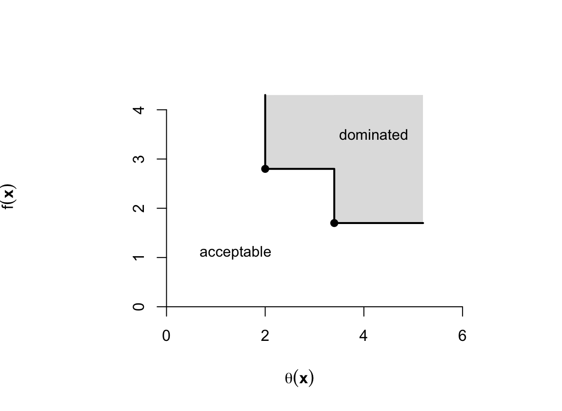
A filter method avoids combining the two objectives with a fixed penalty parameter. It stores pairs (\theta,f) and accepts a new point when it gives sufficient improvement in feasibility or objective value without being dominated by previously accepted pairs.

Figure 1.2: Schematic filter in the (\theta,f) plane. Each accepted pair forbids the quadrant above and to the right of it; a trial point is acceptable only below the resulting staircase, that is, if it improves feasibility or objective value by a sufficient margin.

Even close to a solution, a first-order linearization of curved constraints can cause a merit-function line search to reject the full SQP step. This is the Maratos effect [@maratos1978exact], and it is worth seeing once on a concrete problem rather than taking it on trust.

Example 1.1 (The Maratos effect) Consider

\min_{\bm x\in\mathbb R^2}\; f(\bm x)=2\bigl(x_1^2+x_2^2-1\bigr)-x_1, \qquad h(\bm x)=x_1^2+x_2^2-1=0,

whose solution is \bm x^\star=(1,0)^T: on the circle f=-x_1, which is minimal at x_1=1. From \nabla f(\bm x^\star)=(3,0) and \nabla h(\bm x^\star)=(2,0) the multiplier is \lambda^\star=3/2, so

\bm W_\star=\nabla^2f-\lambda^\star\nabla^2h=4\bm I-3\bm I=\bm I.

Take a feasible iterate on the unit circle,

\bm x_k=(\cos\theta,\sin\theta)^T,

with \theta small, so that h(\bm x_k)=0 and \bm J_k=(2\cos\theta,\,2\sin\theta). The QP of Equation 1.29 minimizes \bm q_k^T\bm p+\tfrac12\|\bm p\|^2 on the tangent line \cos\theta\,p_1+\sin\theta\,p_2=0, and its solution is

\bm p_k=\bigl(\sin^2\theta,\;-\sin\theta\cos\theta\bigr)^T.

It is an excellent step. Since \bm x_k+\bm p_k-\bm x^\star=(1-\cos\theta)(\cos\theta,\sin\theta)^T and \|\bm x_k-\bm x^\star\|^2=2-2\cos\theta,

\|\bm x_k+\bm p_k-\bm x^\star\| =\tfrac12\|\bm x_k-\bm x^\star\|^2,

which is precisely the quadratic rate of Theorem 1.1. Yet the trial point is rejected by any \ell_1 merit function, because

f(\bm x_k+\bm p_k)-f(\bm x_k)=\sin^2\theta>0, \qquad |h(\bm x_k+\bm p_k)|=\sin^2\theta>|h(\bm x_k)|=0.

Both terms of \phi_\rho increase, for every \rho. The line search therefore cuts the step, and the quadratic rate is destroyed by the very mechanism meant to make the method robust.

The cause is that the constraint is curved while the QP sees only its tangent. The standard remedy is a second-order correction: after the step \bm p_k has been computed, solve a second system with the same matrix and the constraint residual re-evaluated at the trial point,

\begin{bmatrix} \bm B_k&-\bm J_k^T\\ -\bm J_k&\bm0 \end{bmatrix} \begin{bmatrix} \widehat{\bm p}\\ \cdot \end{bmatrix} = \begin{bmatrix} \bm0\\ \bm h(\bm x_k+\bm p_k) \end{bmatrix}, \tag{1.41}

and test \bm x_k+\bm p_k+\widehat{\bm p} before shortening the step. In Example 1.1 the correction is \widehat{\bm p}=-\tfrac12\sin^2\theta\,(\cos\theta,\sin\theta)^T+O(\theta^4): it is O(\theta^2), so it does not spoil the quadratic rate, while it reduces the constraint violation from O(\theta^2) to O(\theta^4) and makes the objective decrease. The unit step is then accepted. Because the matrix is unchanged, the extra cost is one back-substitution. Nonmonotone strategies and filters [@fletcher2002nonlinear] are the other standard remedies, and are important for recovering fast local convergence.

Trust-region SQP

Instead of searching along a computed SQP direction, one may restrict the local model to

\|\bm p\|\leq\Delta_k.

The radius is updated using the ratio between actual and predicted reduction [@conn2000trust].

For constrained problems the trust region creates a difficulty that does not arise in the unconstrained case: the linearized constraints \bm h_k+\bm J_k\bm p=\bm0 and the bound \|\bm p\|\le\Delta_k may be jointly infeasible, since a small radius need not contain any point of the linearized feasible set. Shrinking the radius then produces no step at all.

The Byrd–Omojokun decomposition [@omojokun1989trust] resolves this by giving up exact linearized feasibility. The step is split as \bm p=\bm p_N+\bm p_T where the normal step \bm p_N reduces infeasibility as much as the radius permits,

\min_{\bm p_N}\;\|\bm h_k+\bm J_k\bm p_N\|_2 \quad\text{subject to}\quad \|\bm p_N\|\le\zeta\Delta_k, \qquad \zeta\in(0,1),

and the tangential step \bm p_T\in\ker(\bm J_k) then reduces the quadratic model within the remaining radius. The two subproblems are always feasible, \bm p_N=\bm0 and \bm p_T=\bm0 being admissible. This normal–tangential decomposition is the trust-region counterpart of the null-space method for the KKT equations.

Sequential convex methods

The last family of the map in Section 1.2.1 has so far only been named. The idea is the same as SQP, with the quadratic model replaced by any local model that is convex and cheap to solve globally. At \bm x_k one replaces f and the constraints by convex approximations valid in a trust region, solves the resulting convex program to global optimality, and iterates.

Two classical instances are worth distinguishing.

Sequential linear programming [@palacios1982nonlinear] uses a purely linear model, \bm q_k^T\bm p with linearized constraints and a box trust region \|\bm p\|_\infty\le\Delta_k. The subproblem is an LP, which is attractive when a mature LP solver is available and the Hessian is unavailable. The price is that, without curvature, the method is at best linearly convergent unless the solution is a vertex of the linearized feasible set.
Convex–concave procedures and difference-of-convex methods replace each nonconvex term by a convex majorizer, so that every subproblem bounds the true objective from above. Every iterate then improves the objective monotonically, without any line search.

The attraction is that the subproblem has no spurious local minima and the trust region alone provides globalization. The limitation is that the convexified model is generally a weaker local approximation than the exact Lagrangian Hessian, so superlinear convergence is lost unless the model is asymptotically exact. These methods are the natural choice when the problem is nearly convex, when a dedicated convex solver exploits structure that a general QP solver would miss, or when global solvability of each subproblem is itself a requirement.

Primal-dual interior-point Newton system

For inequalities, an interior-point method can first be understood through the logarithmic barrier. With slack variables \bm s=\bm g(\bm x)>\bm0, the barrier subproblem is

\min_{\bm x}\quad f(\bm x)-\tau\sum_{i=1}^{m_g}\log g_i(\bm x), \qquad \tau>0. \tag{1.42}

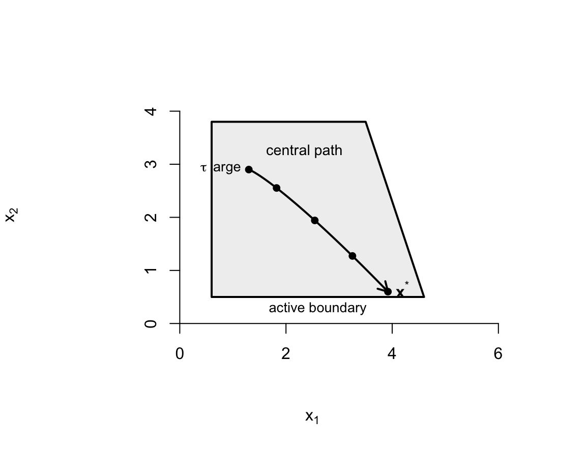
Its stationary points trace the central path as \tau\downarrow0. Introducing multipliers converts the barrier stationarity equations into perturbed complementarity \mu_i s_i=\tau, which leads directly to the primal-dual formulation below.

Figure 1.3: Schematic central path. Barrier minimizers stay strictly feasible for every \tau>0 and approach a KKT point on the boundary as \tau\downarrow0. The markers correspond to decreasing values of the barrier parameter.

Bound constraints

The general NLP Equation 1.18 also carries \bm\ell\le\bm x\le\bm u, and the SQP subproblem Equation 1.35 keeps those bounds explicitly. An interior-point method does not: bounds are inequalities like any other and receive their own slacks, their own multipliers and their own barrier terms. Production codes such as @wachter2006implementation treat them separately only for efficiency, because \partial(\bm x-\bm\ell)/\partial\bm x=\bm I makes the corresponding Jacobian blocks trivial and the resulting diagonal contribution can be added directly to \bm W. In the formulas below the bounds are therefore assumed to have been absorbed into \bm g.

Introduce positive slack variables \bm s through

\bm g(\bm x)-\bm s=\bm0, \qquad \bm s>\bm0,

and positive inequality multipliers \bm\mu>\bm0. Instead of exact complementarity, impose

\bm S\bm\mu=\tau\bm e,

where \bm S=\operatorname{diag}(\bm s) and \tau>0 is the barrier parameter. With \bm M=\operatorname{diag}(\bm\mu), a primal-dual Newton step solves

\begin{bmatrix} \bm W & -\bm J_h^T & -\bm J_g^T & \bm0\\ \bm J_h & \bm0 & \bm0 & \bm0\\ \bm J_g & \bm0 & \bm0 & -\bm I\\ \bm0 & \bm0 & \bm S & \bm M \end{bmatrix} \begin{bmatrix} \Delta\bm x\\ \Delta\bm\lambda\\ \Delta\bm\mu\\ \Delta\bm s \end{bmatrix} =- \begin{bmatrix} \bm r_d\\ \bm r_h\\ \bm r_g\\ \bm r_c \end{bmatrix}, \tag{1.43}

where

\begin{aligned} \bm r_d&=\nabla_x\mathcal L^T,\\ \bm r_h&=\bm h(\bm x),\\ \bm r_g&=\bm g(\bm x)-\bm s,\\ \bm r_c&=\bm S\bm\mu-\tau\bm e. \end{aligned}

Algorithm 3: Basic primal-dual interior-point iteration

Input: \bm x_0, \bm\lambda_0, \bm s_0>0, \bm\mu_0>0, tolerance \varepsilon.

Output: An approximate primal-dual KKT point.

Initialize (\bm x,\bm\lambda,\bm s,\bm\mu)\leftarrow (\bm x_0,\bm\lambda_0,\bm s_0,\bm\mu_0).
Repeat:
1. Form \bm r_d, \bm r_h, \bm r_g and set \eta\leftarrow\bm s^T\bm\mu/m_g.
2. If the primal, dual and complementarity residuals do not exceed \varepsilon, return (\bm x,\bm\lambda,\bm\mu).
3. Set \tau\leftarrow\sigma\eta, with \sigma\in(0,1).
4. Solve Equation 1.43 for (\Delta\bm x,\Delta\bm\lambda,\Delta\bm\mu,\Delta\bm s).
5. Choose fraction-to-the-boundary steps \alpha_p and \alpha_d preserving \bm s+\alpha_p\Delta\bm s>0 and \bm\mu+\alpha_d\Delta\bm\mu>0.
6. Update (\bm x,\bm s) with \alpha_p and (\bm\lambda,\bm\mu) with \alpha_d.
Until the maximum number of iterations is reached.

The basic algorithm displays the central mechanism, but solving the complete four-by-four system directly is rarely the best implementation. The following reductions and predictor–corrector construction are used by practical sparse interior-point solvers.

Eliminating the slack and inequality-multiplier steps

The third block row of Equation 1.43 gives

\Delta\bm s=\bm J_g\Delta\bm x+\bm r_g. \tag{1.44}

Substituting this expression into the complementarity row gives

\Delta\bm\mu = -\bm S^{-1} \left( \bm r_c+\bm M\bm r_g+\bm M\bm J_g\Delta\bm x \right). \tag{1.45}

Eliminating \Delta\bm s and \Delta\bm\mu from the stationarity equation produces the augmented primal Hessian

\bm D = \bm W+\bm J_g^T\bm S^{-1}\bm M\bm J_g. \tag{1.46}

As in the equality-constrained case, multiply the equality-feasibility row by -1. The condensed symmetric-indefinite system, whose coefficient matrix is denoted by \bm K below, is

\begin{bmatrix} \bm D&-\bm J_h^T\\ -\bm J_h&\bm0 \end{bmatrix} \begin{bmatrix} \Delta\bm x\\ \Delta\bm\lambda \end{bmatrix} = \begin{bmatrix} -\bm r_d -\bm J_g^T\bm S^{-1}(\bm r_c+\bm M\bm r_g)\\ \bm r_h \end{bmatrix}. \tag{1.47}

After solving Equation 1.47, recover \Delta\bm s and \Delta\bm\mu from Equation 1.44 and Equation 1.45. This reduction is particularly useful when the number of inequalities is large, because the factorization involves only the primal variables and equality multipliers. In software, the products with \bm S^{-1}\bm M should be formed by diagonal scaling; neither \bm S nor any KKT matrix should be explicitly inverted.

The condensed and full formulations have different numerical tradeoffs. Condensation reduces dimension but can amplify poor scaling when some s_i/\mu_i are very small. A full-space factorization preserves more of the original block structure and can be preferable when the condensed matrix becomes dense.

Fraction-to-the-boundary steps

A Newton direction need not preserve strict positivity. Define

\begin{aligned} \widehat\alpha_p &= \min_{i:\Delta s_i<0} \left(-\frac{s_i}{\Delta s_i}\right),\\ \widehat\alpha_d &= \min_{i:\Delta\mu_i<0} \left(-\frac{\mu_i}{\Delta\mu_i}\right), \end{aligned}

where the minimum of an empty set is +\infty. A fraction-to-the-boundary rule chooses

\alpha_p=\min\{1,\xi\widehat\alpha_p\}, \qquad \alpha_d=\min\{1,\xi\widehat\alpha_d\}, \qquad 0<\xi<1. \tag{1.48}

Values of \xi close to one, such as 0.99 or 0.995, permit rapid progress while keeping \bm s+\alpha_p\Delta\bm s>\bm0 and \bm\mu+\alpha_d\Delta\bm\mu>\bm0. Separate primal and dual step lengths are common; a single step length may be used when a globalization strategy requires it.

Mehrotra predictor–corrector

Mehrotra’s method [@mehrotra1992implementation] estimates how much complementarity a pure Newton step would remove and then chooses the centering parameter adaptively. Let

\eta=\frac{\bm s^T\bm\mu}{m_g}

be the current average complementarity.

The affine-scaling predictor sets \tau=0 and solves the Newton system, producing (\Delta\bm x^{\rm aff},\Delta\bm\lambda^{\rm aff}, \Delta\bm\mu^{\rm aff},\Delta\bm s^{\rm aff}).
Compute maximum affine steps \alpha_p^{\rm aff} and \alpha_d^{\rm aff} that reach, but do not cross, the positivity boundary, and form

\eta_{\rm aff} = \frac{ (\bm s+\alpha_p^{\rm aff}\Delta\bm s^{\rm aff})^T (\bm\mu+\alpha_d^{\rm aff}\Delta\bm\mu^{\rm aff}) }{m_g}.
Select the centering parameter, commonly

\sigma = \left(\frac{\eta_{\rm aff}}{\eta}\right)^3, \qquad \tau=\sigma\eta. \tag{1.49}
The predictor misses the second-order product generated by complementarity. Therefore the corrector solve uses

\bm r_c^{\rm pc} = \bm S\bm\mu +\Delta\bm S^{\rm aff}\Delta\bm\mu^{\rm aff} -\sigma\eta\bm e, \tag{1.50}

where \Delta\bm S^{\rm aff}=\operatorname{diag} (\Delta\bm s^{\rm aff}). The other residuals remain unchanged.

Both solves use the same KKT matrix, so a direct method can reuse the factorization. This is one reason the predictor–corrector method is effective: the second solve is relatively inexpensive.

Algorithm 4: Mehrotra primal-dual predictor–corrector

Input: A strictly positive primal-dual iterate, tolerance \varepsilon, fraction parameter \xi.

Output: An approximate primal-dual KKT point.

Repeat:
1. Form \bm r_d, \bm r_h, \bm r_g and \eta=\bm s^T\bm\mu/m_g.
2. If all scaled KKT residuals are at most \varepsilon, return the current iterate.
3. Solve the affine Newton system with \tau=0.
4. Compute \alpha_p^{\rm aff}, \alpha_d^{\rm aff} and \eta_{\rm aff}.
5. Set \sigma\leftarrow(\eta_{\rm aff}/\eta)^3 and \tau\leftarrow\sigma\eta.
6. Add the second-order term \Delta\bm S^{\rm aff}\Delta\bm\mu^{\rm aff} to the complementarity residual.
7. Solve the corrector system, reusing the KKT factorization.
8. Compute \alpha_p, \alpha_d from Equation 1.48.
9. Update primal and dual variables and recompute the residuals.
Until the iteration limit is reached.

Regularization, inertia, and sparse implementation

On the central path \bm S^{-1}\bm M is positive diagonal. Nevertheless, \bm D need not be positive definite because the Lagrangian Hessian can be indefinite. If \bm D is positive definite on \ker(\bm J_h) and LICQ holds, the symmetric matrix in Equation 1.47 has inertia

\operatorname{inertia}(\bm K) =(n,m_h,0),

namely n positive, m_h negative, and no zero eigenvalues. A sparse LDL^T factorization reveals this inertia. An incorrect inertia signals negative curvature, rank deficiency, or insufficient regularization.

A common stabilized system replaces

\begin{bmatrix} \bm D&-\bm J_h^T\\ -\bm J_h&\bm0 \end{bmatrix} \quad\text{by}\quad \begin{bmatrix} \bm D+\delta_x\bm I&-\bm J_h^T\\ -\bm J_h&-\delta_h\bm I \end{bmatrix}, \tag{1.51}

with small positive \delta_x and \delta_h, increased only when required by factorization stability or inertia. Scaling the rows and columns before factorization is essential, because complementarity can make the diagonal ratios \mu_i/s_i span many orders of magnitude.

For a fixed sparsity pattern, the symbolic ordering of a sparse factorization should be computed once and reused. The affine and corrector solves have the same coefficient matrix, so the numerical factors can also be reused.

Central-path interpretation and convergence

The perturbed KKT mapping is

\bm F_\tau(\bm x,\bm\lambda,\bm\mu,\bm s) = \begin{bmatrix} \nabla_x\mathcal L^T\\ \bm h(\bm x)\\ \bm g(\bm x)-\bm s\\ \bm S\bm\mu-\tau\bm e \end{bmatrix}. \tag{1.52}

At an exact central-path point, \eta=\bm s^T\bm\mu/m_g=\tau. Under LICQ, a second-order sufficient condition, and strict complementarity at the limiting KKT point, the Jacobian of the appropriate primal-dual system is locally nonsingular and the central path approaches that KKT point as \tau\downarrow0.

An implementation does not solve every barrier problem exactly. Instead it keeps the residuals in a neighborhood of the central path while reducing \eta. The affine predictor emphasizes progress toward the boundary; the centering corrector moves the iterate away from an unbalanced boundary approach. Globalization, regularization, and restoration are still required when the starting point is remote, the problem is nonconvex, or the Jacobian is nearly rank deficient; @wachter2006implementation describes a complete filter line-search interior-point method built on these ingredients.

Augmented Lagrangian method

Pure quadratic penalty methods solve

\min_{\bm x} f(\bm x)+\frac{\rho}{2}\|\bm h(\bm x)\|^2.

They require \rho\to\infty to enforce feasibility accurately, which makes the Hessian increasingly ill-conditioned, as Equation 1.23 made explicit. The augmented Lagrangian [@hestenes1969multiplier; @powell1969method; @rockafellar1973dual] avoids this drawback by combining a finite penalty with multiplier estimates:

\mathcal L_\rho(\bm x,\bm\lambda) = f(\bm x) -\bm\lambda^T\bm h(\bm x) +\frac{\rho}{2}\|\bm h(\bm x)\|^2. \tag{1.53}

With the sign convention used here, the multiplier update is

\bm\lambda_{k+1} = \bm\lambda_k-\rho_k\bm h(\bm x_{k+1}). \tag{1.54}

The inner minimization is unconstrained and can be performed with damped Newton, BFGS, or a trust-region method. It need not be solved very accurately at early outer iterations.

Algorithm 5: Method of multipliers

Input: \bm x_0, \bm\lambda_0, penalty \rho_0>0, tolerance \varepsilon.

Output: An approximate KKT pair (\bm x,\bm\lambda).

Set (\bm x,\bm\lambda,\rho)\leftarrow (\bm x_0,\bm\lambda_0,\rho_0).
Repeat:
1. Approximately minimize \mathcal L_\rho(\bm x,\bm\lambda) with respect to \bm x, obtaining \bm x^+.
2. Set \bm\lambda\leftarrow \bm\lambda-\rho\bm h(\bm x^+).
3. If the KKT residual at (\bm x^+,\bm\lambda) does not exceed \varepsilon, return (\bm x^+,\bm\lambda).
4. If feasibility has not decreased sufficiently, set \rho\leftarrow\gamma\rho, with \gamma>1.
5. Tighten the inner-solve tolerance.
6. Set \bm x\leftarrow\bm x^+.
Until the maximum number of outer iterations is reached.

For inequalities \bm g(\bm x)\ge\bm0, the Powell–Hestenes–Rockafellar term compatible with the present sign convention uses

\widehat{\bm\mu}(\bm x) = \max\{\bm0,\bm\mu-\rho\bm g(\bm x)\},

where the maximum is componentwise. The augmented term can be written as

\frac{1}{2\rho} \left( \|\widehat{\bm\mu}(\bm x)\|^2-\|\bm\mu\|^2 \right),

and the multiplier update is

\bm\mu_{k+1} = \max\{\bm0,\bm\mu_k-\rho_k\bm g(\bm x_{k+1})\}.

This projection preserves dual feasibility \bm\mu\ge\bm0.

Why a finite penalty suffices

The quadratic penalty needs \rho\to\infty; the augmented Lagrangian does not. The reason is that Equation 1.54 is a fixed-point iteration in the multipliers, and its contraction factor is O(1/\rho).

Consider the equality-constrained case and suppose LICQ and the second-order sufficient condition hold at (\bm x^\star,\bm\lambda^\star). Two facts follow.

First, there exists a finite threshold \bar\rho such that for every \rho>\bar\rho the point \bm x^\star is a strict local minimizer of \bm x\mapsto\mathcal L_\rho(\bm x,\bm\lambda^\star). Indeed

\nabla^2_{xx}\mathcal L_\rho(\bm x^\star,\bm\lambda^\star) = \bm W_\star+\rho\,\bm J_\star^T\bm J_\star, \tag{1.55}

and \bm W_\star is positive definite on \ker(\bm J_\star) while \rho\bm J_\star^T\bm J_\star supplies positive curvature on the complementary subspace. For \rho large enough the sum is positive definite on all of \mathbb R^n. The exact multiplier therefore converts the constrained problem into an unconstrained one without any limit.

Second, if \bm x(\bm\lambda) denotes the local minimizer of \mathcal L_\rho(\cdot,\bm\lambda), the update \bm\lambda^{+}=\bm\lambda-\rho\bm h(\bm x(\bm\lambda)) satisfies

\|\bm\lambda^{+}-\bm\lambda^\star\| \le \frac{C}{\rho}\,\|\bm\lambda-\bm\lambda^\star\| \tag{1.56}

for a constant C independent of \rho. Convergence of the outer iteration is therefore linear, with a rate that can be made as small as desired by increasing \rho — but the required \rho is finite and fixed, so the conditioning of Equation 1.55 stays bounded. This is the whole point of the method, and it is why the penalty is increased in the algorithm only when feasibility fails to improve, never as a matter of course.

The price is the rate: linear, against the quadratic rate of SQP. Augmented Lagrangian methods are therefore preferred when the inner problem has exploitable structure, when feasibility is hard to attain, or when bound constraints can be handled directly in the inner solve [@conn1991globally], rather than when fast local convergence is the priority.

A worked example

Everything above is easier to trust after seeing it run. Consider the smallest nontrivial equality-constrained problem,

\min_{\bm x\in\mathbb R^2}\; f(\bm x)=-x_1-x_2 \qquad\text{subject to}\qquad h(\bm x)=x_1^2+x_2^2-1=0, \tag{1.57}

whose solution is immediate: on the unit circle f=-x_1-x_2 is minimal at

\bm x^\star=\tfrac{1}{\sqrt2}(1,1)^T, \qquad \lambda^\star=-\tfrac{1}{\sqrt2}\approx-0.7071,

since \bm q=(-1,-1)^T and \bm J_\star=\sqrt2\,(1,1) give \bm q=\bm J_\star^T\lambda^\star. The Lagrangian Hessian is

\bm W=\nabla^2f-\lambda\nabla^2h=-2\lambda\,\bm I,

so at the solution \bm W_\star=\sqrt2\,\bm I\succ\bm0 and the second-order sufficient condition Equation 1.30 holds.

The objective Hessian alone would fail here

Note that \nabla^2f=\bm0. Replacing \bm W by \nabla^2f, as warned against in the discussion preceding Equation 1.34, would make the KKT matrix

\begin{bmatrix}\bm0&-\bm J^T\\-\bm J&\bm0\end{bmatrix}

singular: the method would not merely converge more slowly, it would not produce a step at all. The same happens if the iteration is started with \lambda_0=0. All the curvature of this problem lives in the constraint.

The following implements Equation 1.25 literally — assemble, solve, update — with no globalization, starting from an infeasible point \bm x_0=(0.6,0.9)^T and \lambda_0=-1.

q  <- function(x) c(-1, -1)              # objective gradient (column)
Hf <- function(x) matrix(0, 2, 2)        # objective Hessian
h  <- function(x) x[1]^2 + x[2]^2 - 1    # constraint
Jh <- function(x) matrix(c(2 * x[1], 2 * x[2]), nrow = 1)
Hh <- function(x) 2 * diag(2)            # constraint Hessian

xstar <- c(1, 1) / sqrt(2)

x <- c(0.6, 0.9)
lam <- -1
rows <- list()

for (k in 0:5) {
  J  <- Jh(x)
  W  <- Hf(x) - lam * Hh(x)              # Lagrangian Hessian
  rd <- q(x) - as.vector(t(J)) * lam     # dual residual
  rows[[k + 1]] <- data.frame(
    k        = k,
    err      = sqrt(sum((x - xstar)^2)),
    kkt      = max(abs(rd), abs(h(x))),
    lambda   = lam
  )
  K   <- rbind(cbind(W, -t(J)), cbind(-J, 0))   # symmetric indefinite
  d   <- solve(K, c(-rd, h(x)))                 # (p, delta lambda)
  x   <- x + d[1:2]
  lam <- lam + d[3]
}

tab <- do.call(rbind, rows)
knitr::kable(
  data.frame(
    k        = tab$k,
    error    = sprintf("%.3e", tab$err),
    residual = sprintf("%.3e", tab$kkt),
    lambda   = sprintf("%.8f", tab$lambda)
  ),
  col.names = c("$k$", "$\\lVert\\bm x_k-\\bm x^\\star\\rVert$",
                "$\\lVert\\bm F(\\bm z_k)\\rVert_\\infty$", "$\\lambda_k$"),
  align = "rrrr", booktabs = TRUE, escape = FALSE
)

Table 1.1: Exact-Hessian SQP on Equation 1.57. The number of correct digits doubles at each iteration, as predicted by Theorem 1.1.

k	\lVert\bm x_k-\bm x^\star\rVert	\lVert\bm F(\bm z_k)\rVert_\infty	\lambda_k
0	2.206e-01	8.000e-01	-1.00000000
1	6.169e-02	8.149e-02	-0.71367521
2	1.959e-03	3.689e-03	-0.70587593
3	2.236e-06	4.349e-06	-0.70710317
4	6.405e-12	1.568e-11	-0.70710678
5	1.110e-16	2.220e-16	-0.70710678

The error goes from 6\cdot10^{-2} to 2\cdot10^{-3} to 2\cdot10^{-6} to 6\cdot10^{-12}: each iteration roughly squares the previous error, which is Equation 1.31 in action. Machine precision is reached in five iterations, and the multiplier converges at the same rate as the primal variables — it is a component of \bm z, not an afterthought.

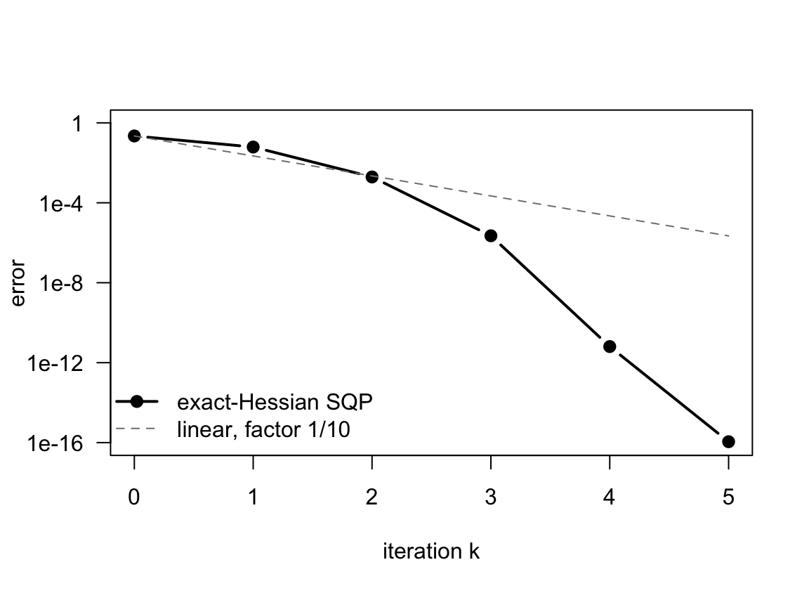
Figure 1.4: Quadratic convergence of exact-Hessian SQP on Equation 1.57. On a logarithmic scale a quadratic rate is a curve whose slope doubles, not a straight line; the dashed reference line is linear convergence with factor 1/10.

Two remarks close the example. The iteration above has no line search, no merit function and no trust region: near the solution none is needed, and a correctly implemented globalization must become inactive exactly here, or the rate shown in Table 1.1 is lost — which is precisely what Example 1.1 illustrates. And the entire method is six lines of linear algebra; the difficulty of constrained optimization lies in making those six lines survive a bad starting point, not in the lines themselves.

Exercises

Exercises 1–3 are fundamental, 4–6 computational, and 7–10 advanced. Starting hints: use block elimination for 1–2; inspect the penalty Hessian spectrum for 3–4; retain second-order terms for 5; compare reduced and full KKT residuals for 6; preserve positivity during elimination for 7–8; and use regularization or a better multiplier estimate for 9–10.

Row scaling. Show that multiplying the second block row of Equation 1.26 by -1 changes neither the Newton step nor the solution set, and that the resulting matrix is symmetric. Why is a Cholesky factorization still inapplicable?
Inertia. Let \bm K be the matrix of Equation 1.25 with \bm J of full row rank m_h. Prove that if \bm Z^T\bm W\bm Z\succ\bm0 then \operatorname{inertia}(\bm K)=(n,m_h,0). Deduce a practical test for second-order sufficiency from a sparse LDL^T factorization.
Penalty conditioning. For Equation 1.57 write the Hessian of the quadratic penalty Equation 1.21 at the solution and compute its condition number as a function of \rho. Compare with Equation 1.55 for the augmented Lagrangian with the exact multiplier.
The multiplier hidden in the penalty. Minimize Equation 1.21 numerically for \rho=10,10^2,\dots,10^6 and verify Equation 1.23 against \lambda^\star=-1/\sqrt2. At which \rho does the estimate stop improving, and why?
Maratos. Reproduce Example 1.1 numerically for \theta=10^{-1},10^{-2},10^{-3}: compute \bm p_k, verify that both f and |h| increase, then compute the second-order correction Equation 1.41 and check that the full step becomes acceptable.
Null-space versus full space. Solve the QP of Equation 1.57 by the reduced system Equation 1.37, recover the multiplier from Equation 1.38, and check that the result agrees with the full KKT solve of Table 1.1 to machine precision.
Interior point by hand. Replace the equality in Equation 1.57 by 1-x_1^2-x_2^2\ge0. Write the system Equation 1.43, perform the elimination of Equation 1.44 and Equation 1.45 explicitly, and verify that the condensed matrix is the one in Equation 1.47. Trace the central path for \tau=10^{-1},\dots,10^{-6}.
Fraction to the boundary. Show that Equation 1.48 with \xi<1 guarantees \bm s>\bm0 and \bm\mu>\bm0 after the update, and explain why \xi=1 would be unsafe even though the iterate would remain nonnegative.
Quasi-Newton. Replace \bm W in the worked example by a BFGS matrix updated with Equation 1.39 and the Lagrangian-gradient difference. Measure the observed rate and check it against the Dennis–Moré condition.
Degenerate multiplier. Explain why starting the worked example with \lambda_0=0 makes the first KKT matrix singular, and propose two remedies consistent with the regularization discussed above.

Local convergence and regularity

Fast local convergence requires more than smoothness. The standard assumptions that repeatedly appear in NLP analysis are:

a constraint qualification, typically LICQ, so that the relevant constraint Jacobian has full row rank;
a second-order sufficient condition, meaning that the Lagrangian Hessian is positive definite on the critical or tangent subspace;
for the cleanest inequality-constrained local theory, strict complementarity or an appropriate weaker nondegeneracy assumption;
sufficiently accurate derivative information and linear solves.

Under these assumptions, exact Newton applied to the equality-constrained KKT system is locally quadratically convergent. Exact-Hessian SQP inherits this rate once the correct active structure is identified and unit steps are accepted. Quasi-Newton SQP can be superlinear when the Hessian approximation satisfies an appropriate Dennis–Moré condition on the relevant subspace.

Global convergence has a different meaning: it normally asserts that, from a sufficiently broad set of starting points, accumulation points are stationary or satisfy first-order KKT conditions. It does not imply convergence to a global minimizer for a nonconvex NLP. Merit functions, filters, trust regions, restoration phases, and penalty/barrier updates are devices for obtaining this kind of globalization.

Infeasible starts and restoration

Requiring a feasible initial point can itself be as difficult as the original NLP. Modern SQP and interior-point solvers therefore commonly permit infeasible iterates [@gill2005snopt; @wachter2006implementation]. If the main step cannot make acceptable progress, a restoration phase approximately solves a feasibility problem such as

\min_{\bm x}\quad \|\bm h(\bm x)\|_1+ \|\min\{\bm g(\bm x),\bm0\}\|_1,

possibly subject to simple bounds or a trust region. The objective of the restoration phase is not to optimize f, but to return to a region where the main NLP model is meaningful.

Linear algebra for KKT systems

The linear solve is usually the dominant cost of a constrained optimization iteration. Several formulations are useful.

Symmetric-indefinite factorization. Sparse LDL^T factorization with pivoting is the standard robust choice for a moderate-size KKT matrix.
Null-space method. If \bm Z spans \ker(\bm J), compute the tangential step from the reduced Hessian \bm Z^T\bm W\bm Z. This is attractive when the number of constraints is small.
Range-space or Schur-complement method. Eliminate the primal step and solve a system in the multipliers. This is effective when solves with \bm W are cheap.
Iterative methods. For very large sparse problems, MINRES or GMRES with block preconditioning avoids a complete factorization.

Scaling is essential: badly scaled variables or constraints can make an otherwise regular KKT matrix appear nearly singular. Regularization of both the primal and multiplier blocks is common in production solvers.

Stopping criteria and diagnostics

For equality constraints, a natural scaled KKT measure is

\mathcal E_{\mathrm{eq}} = \max\left\{ \frac{\|\nabla_x\mathcal L^T\|_\infty}{1+\|\bm\lambda\|_\infty}, \|\bm h(\bm x)\|_\infty \right\}.

For inequalities, monitor four distinct quantities:

\begin{aligned} \text{stationarity:}\quad &\|\nabla_x\mathcal L^T\|_\infty,\\ \text{equality feasibility:}\quad &\|\bm h(\bm x)\|_\infty,\\ \text{inequality violation:}\quad &\|\min(\bm g(\bm x),\bm0)\|_\infty,\\ \text{complementarity:}\quad &\|\min\{\bm\mu,\bm g(\bm x)\}\|_\infty. \end{aligned}

The last measure deserves a comment. The product \|\bm\mu\odot\bm g\|_\infty is the obvious candidate, but it is misleading on infeasible iterates: if g_i<0 and \mu_i is small, the product is tiny although neither feasibility nor complementarity holds. The natural residual \min\{\mu_i,g_i\} vanishes if and only if \mu_i\ge0, g_i\ge0 and \mu_ig_i=0, so it measures dual feasibility, primal feasibility and complementarity at once. All residuals should be scaled, for example by 1+\|\bm\lambda\|_\infty for stationarity and by a characteristic constraint magnitude for feasibility.

A small step is not, by itself, evidence of convergence: it may instead indicate a failed line search, a singular KKT matrix, poor scaling, or an incorrect active set. A reliable implementation reports all primal, dual, and complementarity residuals separately.

Choosing a method

Problem structure	Suitable first choice
Smooth unconstrained, accurate Hessian available	Damped Newton or trust-region Newton
Smooth unconstrained, expensive Hessian	BFGS or limited-memory BFGS
Equality constraints, moderate sparse system	Newton–SQP with sparse LDL^T
Few active inequalities	Active-set SQP
Many large sparse inequalities	Primal-dual interior-point method
Simple convex set or box constraints	Projected gradient/Newton or bound active set
Difficult initial feasibility or decomposable inner solves	Augmented Lagrangian method
Convex local approximations are natural	Sequential convex programming

No method removes the need for good scaling, accurate derivatives, and a globalization strategy. These three ingredients often matter more in practice than the distinction between closely related Newton-type variants.

A practical hierarchy for smooth NLP

For a smooth constrained problem, the following hierarchy is useful when selecting or designing a numerical method.

Exploit simple constraints directly: eliminate fixed variables and use projections for boxes or other cheaply projectable convex sets.
For general smooth constraints, regard the KKT equations as the local target and decide whether active-set/SQP or interior-point treatment of inequalities is more appropriate.
Use the exact Lagrangian Hessian when it is affordable and reliable; otherwise use BFGS, limited-memory approximations, or matrix-free Hessian-vector products.
Globalize the local step with a merit function, filter, or trust region.
Use augmented-Lagrangian or restoration mechanisms when feasibility is particularly difficult.
Measure convergence with primal feasibility, dual stationarity, and complementarity residuals rather than with the step norm alone.

This hierarchy emphasizes a central theme: modern constrained optimization is largely the numerical linear algebra of KKT systems combined with a mechanism for deciding which KKT system to solve and how much of its Newton step to accept.