University of Trento, Department of Industrial Engineering
The explicit Euler method was obtained in the previous chapter by truncating the Taylor expansion of the exact solution after the linear term. Nothing forces us to stop there: if the solution is smooth enough, keeping more terms produces a one-step method of arbitrarily high order. The resulting family, the Taylor methods, is the natural reference against which Runge–Kutta methods are judged, and it is the only elementary way to reach high order using the information available at a single point.
Throughout this chapter we consider the scalar initial value problem
t_k = a+kh,
\qquad
h = \frac{b-a}{N},
\qquad
k=0,1,\ldots,N,
and we assume that f has as many continuous partial derivatives as the expansions below require. The extension to systems is purely notational: every derivative becomes a vector and every partial derivative a Jacobian or a higher-order tensor.
3.1 Taylor Methods of Low Order
The three lowest-order Taylor methods are built the same way: truncate the Taylor expansion of the solution and replace the derivatives by their expressions in terms of f. Order one gives Euler, and each further term costs one more total derivative.
Neglecting the \mathcal O(h^2) remainder yields the explicit Euler method
y_{k+1}=y_k+h f(y_k,t_k),
whose local truncation error is \mathcal O(h^2) and whose global order is therefore one. The question addressed here is what happens when the remainder is pushed one or more orders further.
raises an immediate difficulty: y''(t_k) is not directly available. It is, however, completely determined by the differential equation. Differentiating y'(t)=f(y(t),t) with respect to t and using the chain rule,
Building a Taylor method of order p requires the partial derivatives of f up to order p-1. Computing them by hand is laborious and error prone already for p=3. In practice one relies on a computer algebra system (Mathematica, Maple, SymPy) or on automatic differentiation, which evaluates the derivatives to machine accuracy without producing their symbolic expressions. The recursive formulation of Section 3.2 is precisely what such tools implement.
The Third-Order Taylor Method
One further term requires y'''. Differentiating the expression just obtained for y'',
with all quantities now evaluated at the numerical point (y_k,t_k).
ImportantThe cost of order
Comparing Equation 3.2 and Equation 3.3 shows the structural weakness of the family: the number of elementary differentials grows combinatorially with the order (1, 2, 5, 15, … terms for orders 1, 2, 3, 4, …), exactly as the number of rooted trees in the Runge–Kutta order conditions. Each of them involves a different partial derivative of f.
Runge–Kutta methods were invented to buy the same order without any derivative of f, paying instead with a few extra evaluations of f per step. This is the comparison that motivates the next chapter.
3.2 A Recursive Formulation
The derivations above are instances of a single recursion that can be carried out to any order. Let y solve y'=f(y,t) and consider the Taylor expansion
Using these six functions in Equation 3.6 produces a sixth-order method for this particular equation. Note how quickly the expressions grow even for a right-hand side as simple as a bilinear polynomial: this growth is the price of eliminating y' at every stage of the recursion.
3.3 An Improved Recursion
The explosion observed above is largely an artefact of insisting that D_k depend on (y,t) only. Each substitution y'\mapsto f(y,t) is immediately followed by a differentiation, which reintroduces the same subexpressions in a more complicated form.
If instead the derivatives already computed are kept as independent arguments, the recursion stays simple. Consider
with the convention y^{(0)}=y. The derivatives y'_k,y''_k,\ldots are evaluated in sequence at each mesh point, so the right-hand side of the recurrence is always available.
Example: f(y,t)=t+y+ty Revisited
For the same equation, and omitting the arguments,
Each derivative now costs a couple of arithmetic operations instead of the evaluation of a polynomial of growing degree: the same sixth-order accuracy is obtained at a small fraction of the cost of Equation 3.6.
Numerical Check of the Order
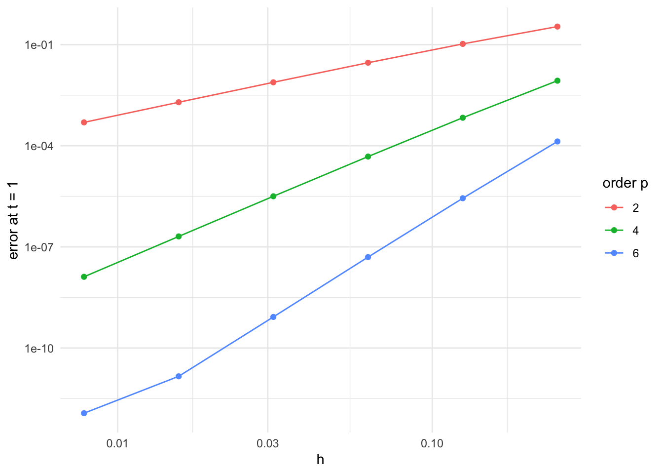
The following experiment integrates y'=t+y+ty with y(0)=1 on [0,1] using the improved recursion truncated at orders p=2,4,6, and compares the error at t=1 against the reference solution produced by a stringent adaptive solver.
taylor_step <-function(t, y, h, p) { d <-numeric(p) # d[j] = y^(j) d[1] <- (t +1) * y + tif (p >=2) d[2] <- (t +1) * d[1] + y +1if (p >=3) for (k in3:p) d[k] <- (t +1) * d[k-1] + (k-1) * d[k-2] y +sum(h^(1:p) /factorial(1:p) * d)}taylor_solve <-function(N, p, t0 =0, y0 =1, T =1) { h <- (T - t0) / N; t <- t0; y <- y0for (k in1:N) { y <-taylor_step(t, y, h, p); t <- t + h } y}# reference solution: y' = (1+t) y + t, solved to near machine accuracyref <- deSolve::ode(y =1, times =c(0, 1),func =function(t, y, parms) list((1+ t) * y + t),parms =NULL, rtol =1e-14, atol =1e-14)[2, 2]Ns <-2^(2:7)err <-expand.grid(N = Ns, p =c(2, 4, 6))err$error <-mapply(function(N, p) abs(taylor_solve(N, p) - ref), err$N, err$p)err$h <-1/ err$Ntab <- reshape2::dcast(err, N ~ p, value.var ="error")tab[-1] <-lapply(tab[-1], formatC, format ="e", digits =2)knitr::kable( tab,col.names =c("$N$", "$p=2$", "$p=4$", "$p=6$"),align ="r",caption ="Absolute error at $t=1$ as a function of the number of steps.")
Absolute error at t=1 as a function of the number of steps.
N
p=2
p=4
p=6
4
3.44e-01
8.51e-03
1.34e-04
8
1.05e-01
6.77e-04
2.77e-06
16
2.90e-02
4.78e-05
4.98e-08
32
7.62e-03
3.17e-06
8.35e-10
64
1.95e-03
2.04e-07
1.44e-11
128
4.94e-04
1.30e-08
1.16e-12
# observed orders from consecutive refinementsord <-do.call(rbind, lapply(c(2, 4, 6), function(p) { e <- err$error[err$p == p]data.frame(p = p, observed =c(NA, log2(head(e, -1) /tail(e, -1))))}))ord$N <-rep(Ns, times =3)
ggplot2::ggplot(err, ggplot2::aes(h, error, colour =factor(p))) + ggplot2::geom_line() + ggplot2::geom_point() + ggplot2::scale_x_log10() + ggplot2::scale_y_log10() + ggplot2::labs(x ="h", y ="error at t = 1", colour ="order p") + ggplot2::theme_minimal()
Figure 3.1: Error at t=1 for the Taylor methods of order 2, 4 and 6.
knitr::kable( reshape2::dcast(ord, N ~ p, value.var ="observed"),col.names =c("$N$", "$p=2$", "$p=4$", "$p=6$"),digits =3, align ="r",caption ="Observed order $\\log_2(e_{N}/e_{2N})$ between consecutive refinements.")
Observed order \log_2(e_{N}/e_{2N}) between consecutive refinements.
N
p=2
p=4
p=6
4
NA
NA
NA
8
1.709
3.652
5.595
16
1.856
3.826
5.799
32
1.929
3.913
5.898
64
1.965
3.957
5.853
128
1.983
3.978
3.633
The observed slopes approach the nominal orders 2, 4 and 6. The last entry of the sixth-order column degrades not because the method fails, but because the error has reached the accuracy of the reference solution itself: with p=6 and N=128 the approximation is already as good as the yardstick used to measure it. This is the usual warning that an order verification is meaningful only in the window between the pre-asymptotic transient and the accuracy floor of the comparison.
Summary
Repeated differentiation of the ODE expresses y'', y''', … in terms of f and its partial derivatives; truncating the Taylor series at order p gives a one-step method of order p.
The method reaches any order using information at a single point, but requires the derivatives of f: it is practical only with symbolic or automatic differentiation.
The recursion Equation 3.5 is the straightforward formulation; the improved recursion Equation 3.7 keeps the previously computed derivatives as arguments and avoids the combinatorial growth of the expressions.
The comparison is what motivates Runge–Kutta methods: the same order, no derivatives of f, at the price of several evaluations of f per step.