University of Trento, Department of Industrial Engineering
In many cases, finding an analytical solution to initial value problems (IVPs) is either impossible or impractical due to the complexity of the integrals involved. Therefore, numerical methods are commonly used to approximate solutions. These methods can be applied not only to single IVPs but also extend naturally to systems of differential equations. Additionally, since higher-order differential equations can be reformulated as systems of first-order equations, we will focus on numerical methods for first-order systems.
Definition 2.1 (Time Discretization) On a time interval I=[t_0,t_0+T], introduce a mesh
t_0<t_1<\cdots<t_N=t_0+T.
The k-th time step is the subinterval
I_k=[t_k,t_{k+1}],
\qquad k=0,1,\ldots,N-1,
with step size
h_k=t_{k+1}-t_k>0.
For a uniform mesh, h_k=h=T/N for every k. Using N for the number of time steps avoids confusing it with the dimension of the ODE system.
Numerical methods for solving IVPs are divided into two primary categories: one-step methods and multi-step methods. In one-step methods, the next approximation z_{k+1} depends only on the current step z_k. In contrast, multi-step methods calculate z_{k+1} using information from several previous time levels. The number of previous levels (the number of steps) must not be confused with the order of accuracy of the method.
Definition 2.2 (One-Step Methods)
Explicit Methods
An explicit method (also called forward integration) calculates approximations sequentially. Starting with an initial condition z_0 at time t_0, it computes the sequence z_1, z_2, \dots, z_n using the following update formula:
Here, \bm{F} is called the increment function, which determines the change from one time step to the next. Here p+1 indicates how many previously computed states enter the increment function; it is not the order of accuracy. A one-step method depends only on \bm{z}_k.
Definition 2.3 (Implicit Methods) An implicit method (also called backward integration) is similar in structure to explicit methods but requires solving for the new value z_{k+1} implicitly. The update formula is given by:
In this case, the increment function \bm{F} depends on \bm{z}_{k+1}, meaning the equation must be solved iteratively or using numerical techniques to find \bm{z}_{k+1}. Implicit methods often provide better stability, especially for stiff differential equations, but are computationally more intensive because of the need to solve for \bm{z}_{k+1} at each step.
In summary, the distinction between explicit and implicit methods is primarily in how the next step is computed. Explicit methods are generally simpler but may require smaller time steps for stability, whereas implicit methods can handle larger time steps but at the cost of increased computational effort.
2.1 A First Look at the Explicit Euler Method
Before introducing the general convergence theory for one-step methods, it is useful to see the complete argument in the simplest possible setting. We therefore consider first the scalar initial value problem
Geometrically, at every point (t_k,y_k) the method follows for one time step the tangent line whose slope is f(y_k,t_k). The new point is then used to compute the tangent for the following step.
A Direct Error Estimate for Euler
The preceding derivation suggests that the error made in one step is of order h^2. We now show directly how these one-step errors accumulate.
Let
e_k=y(t_k)-y_k
be the global error. Taylor’s theorem with Lagrange remainder gives
The next theorem abstracts exactly this argument and applies it to a general one-step method.
Consistency, Local Error, and Convergence
A large class of one-step methods can be written as
\bm{z}_{k+1}=\bm{z}_k+h\,\bm\Phi(t_k,\bm{z}_k;h),
where \bm\Phi is the increment function. To discuss accuracy, it is useful to distinguish the error made in one exact step from the error accumulated over many steps.
Definition 2.4 (Local Defect and Order) Let \bm{z}(t) be the exact solution. The local defect is
The distinction is essential: a local defect O(h^{p+1}) is produced at each of approximately T/h steps, so one expects a global error O(h^p) provided perturbations are not amplified too strongly.
Theorem 2.1 (Convergence Theorem for One-Step Methods) Assume that, for 0<h\le h_0, the increment function is uniformly Lipschitz in the state variable,
Note the structure of the bound: the local defects accumulate, and the accumulation is amplified by the factor e^{L_\Phi(t_k-t_0)}. This is exactly the amplification of the continuous-dependence estimate obtained from Grönwall’s lemma — same structure, same reason. The constant degrades exponentially with the length of the integration interval, which is why a global error bound of this type is informative on a fixed interval and essentially useless for long-time integration.
TipWhere L_\Phi comes from
For explicit Euler \bm\Phi=\bm{f}, so L_\Phi=L, the Lipschitz constant of \bm{f}. For a multistage method \bm\Phi is a composition of evaluations of \bm{f} and one obtains L_\Phi=L\bigl(1+\mathcal O(hL)\bigr). The Lipschitz property of \bm{f} is therefore the only substantial hypothesis — the same one that guarantees existence and uniqueness of the solution, Picard–Lindelöf theorem. Without it there is neither a unique solution to approximate nor a convergence statement to prove.
WarningWhat the theorem does not say
The estimate holds as h\to0 on a fixed interval. It says nothing about the behaviour as k\to\infty at fixed h: that is the subject of absolute stability, a property entirely independent of the order p. A method of order four can produce a numerical solution that grows without bound on a stiff problem, and the convergence theorem is not violated — it simply does not apply to that regime.
2.2 Euler Method in Vector Form
The Euler method is the simplest one-step numerical method for solving initial value problems (IVPs). One intuitive way to derive this method is through the truncated Taylor series expansion.
where \bm{z}'(t_0) = \bm{f}(\bm{z}_0,t_0). Neglecting higher-order terms, we approximate \bm{z}(t_0 + \Delta t) as:
\bm{z}(t_0 + \Delta t) \approx \bm{z}(t_0) + \Delta t \bm{z}'(t_0),
The difference between this approximation and the exact solution \bm{z}(t_0 + \Delta t) is proportional to \Delta t^2, meaning the error decreases as \Delta t becomes smaller.
General Form of the Euler Method
To generalize this for any time interval I = [t_0, t_0 + T], we divide the interval into subintervals and apply the approximation at each step. For the k-th subinterval
I_k = [t_{k-1}, t_k]
the explicit Euler method for the k-th step is given by:
\bm{z}_{k+1} = \bm{z}_k + \Delta t\bm{f}(\bm{z}_k,t_k), \quad k = 0,1,\dots,n-1,
and sets \bm{w}^{(m+1)}=\bm{w}^{(m)}+\bm{s}^{(m)}; the inverse is not formed explicitly. A natural initial guess is the explicit Euler predictor
\bm{w}^{(0)}=\bm{z}_k+h\bm{f}(\bm{z}_k,t_k).
The nonlinear iteration should be stopped when both the residual and/or the Newton correction are sufficiently small relative to the requested ODE accuracy. Solving the nonlinear system much more accurately than the time-discretization error is usually unnecessary.
Convergence and Stability
Both the explicit and implicit Euler methods are first-order accurate, meaning that their local truncation error is \mathcal{O}(\Delta t^2), leading to a global error that scales as \mathcal{O}(\Delta t). As the step size \Delta t\to 0, both methods converge to the exact solution, with the error at any time
t \in I = [t_0, t_0 + T],
bounded by C \Delta t, where C is a constant. However, in practice, this constant can grow exponentially with T, following
C \propto e^{L T},
where L is the Lipschitz constant of the function \bm{f}(\bm{z},t). This growth in error amplification is particularly problematic for large-time integration.
Local and global error
For a one-step method, the local truncation error is the defect produced by one step when the exact value is supplied at the beginning of the step. The global error is
\bm{e}_k=\bm{z}(t_k)-\bm{z}_k.
For explicit Euler, if \bm{z}\in C^2 and \bm{f} is Lipschitz in \bm{z} with constant L, Taylor’s theorem gives a local defect bounded by C_0h^2. The error recursion satisfies
\|\bm{e}_{k+1}\|\le(1+hL)\|\bm{e}_k\|+C_0h^2.
Iterating this inequality and using (1+hL)^k\le e^{L(t_k-t_0)} yields
for L>0 (with the obvious limit C_0(t_k-t_0)h when L=0). This proves first-order convergence on every fixed finite interval.
Stability Considerations
One of the key differences between the explicit and implicit Euler methods lies in their stability properties. The explicit Euler method has a stability constraint dictated by the step size \Delta t, requiring \Delta t to be sufficiently small to ensure numerical stability. Specifically, for a linear test equation of the form
the explicit Euler method is stable only if h satisfies the stability condition:
|1 + \Delta t\lambda| \leq 1.
For stiff problems, where solutions evolve on vastly different time scales and exhibit rapid transient dynamics, this condition can impose severely restrictive time-step limitations, making explicit Euler impractical.
In contrast, the implicit Euler method has stability function R(q)=1/(1-q), q=\Delta t\,\lambda. Its absolute-stability region contains the entire left half-plane: it is therefore A-stable. Moreover R(q)\to0 as |q|\to\infty in the left half-plane, so implicit Euler is also L-stable. “Unconditionally stable” should only be understood in this precise test-equation sense, not as a statement that every numerical problem is stable for arbitrary step sizes. This property makes it particularly advantageous for stiff problems, where it allows for significantly larger time steps without numerical instability. However, this comes at the cost of solving a nonlinear equation at each step, increasing computational expense.
Thus, while both methods share the same convergence rate of \mathcal{O}(\Delta t), their stability properties determine their applicability:
Explicit Euler: Suitable for non-stiff problems but requires small \Delta t for stability.
Implicit Euler: More robust for stiff problems, allowing larger \Delta t, but requires solving implicit equations at each step.
What is stiffness?
There is no single definition of stiffness that covers every nonlinear problem, but the computational phenomenon is clear: a problem is called stiff when stability, rather than accuracy, forces an explicit method to use a step size much smaller than the time scale on which the solution of interest changes.
For the linear system
\bm{z}'=\bm{A}\bm{z},
suppose the eigenvalues of \bm{A} have negative real parts. Each eigenmode behaves approximately like e^{\lambda_i t}. If some modes decay extremely rapidly while others decay slowly, an explicit method must resolve the fastest stable mode even after that transient has become negligible.
When all relevant eigenvalues are real and negative, the heuristic stiffness ratio
measures the separation of decay time scales. A large value is an indication of stiffness, not a universal definition. For general non-normal or nonlinear systems, eigenvalues alone may not capture the whole phenomenon.
This explains why A-stable and especially L-stable implicit methods are useful: they can strongly damp rapidly decaying modes without forcing h to resolve their shortest time scale.
2.3 Stability: continuous problem versus numerical method
The word stability is used for several distinct concepts. Keeping them separate prevents a common source of confusion.
Stability of the continuous IVP
For two exact solutions of
\bm{z}'=\bm{f}(\bm{z},t),
with nearby initial data, continuous dependence gives, under a Lipschitz assumption,
This is a property of the differential equation, not of a discretization.
Zero-stability and propagation of perturbations
A numerical method is also affected by perturbations: roundoff, inexact nonlinear solves, perturbed starting values, and local truncation errors. For one-step methods, a Lipschitz bound on the increment function provides the required finite-time stability. For linear multistep methods the corresponding concept is zero-stability, treated in the dedicated chapter.
Absolute stability
Absolute stability addresses a different question: whether a numerical method reproduces the decay of the scalar test problem
z'=\lambda z,
\qquad \operatorname{Re}\lambda<0.
If a method gives
z_{n+1}=R(q)z_n,
\qquad q=h\lambda,
its absolute-stability region is
\mathcal S=\{q\in\mathbb C:|R(q)|\le1\}.
This is a property of the numerical method applied to the test equation; it is not the same as convergence or stability of the exact IVP.
A-stability and L-stability
A method is A-stable if
\{q\in\mathbb C:\operatorname{Re}q\le0\}\subseteq\mathcal S.
Thus every exponentially decaying scalar mode is numerically stable for every step size. A method is L-stable if it is A-stable and additionally
L-stability is especially useful for stiff problems because very fast stable modes are strongly damped rather than merely kept bounded.
These notions form a hierarchy of different questions:
well-posedness / continuous dependence concerns the exact ODE;
consistency measures the one-step defect of the discretization;
zero-stability or one-step stability controls perturbation growth;
convergence asks whether the numerical solution approaches the exact one as h\to0;
absolute, A-, and L-stability describe behavior for decaying test modes at finite step size.
2.4 Heun and Collatz Methods
Heun’s Method
Heun’s method, also known as the improved Euler method, is a second-order numerical method for solving initial value problems (IVPs). It refines the accuracy of the explicit Euler method by incorporating an additional correction step.
This two-stage approach makes Heun’s method more accurate than explicit Euler, achieving a global error of \mathcal{O}(\Delta t^2) instead of \mathcal{O}(\Delta t).
Convergence and Stability
Heun’s method is second-order accurate, meaning that its local truncation error is \mathcal{O}(\Delta t^3), leading to a global error of \mathcal{O}(\Delta t^2). Compared to the explicit Euler method, it provides improved accuracy for the same step size.
In terms of absolute stability, Heun’s method is conditionally stable. For the scalar test equation its stability polynomial is
R(q)=1+q+\frac{q^2}{2}.
Along the negative real axis the stability interval is again [-2,0], exactly as for explicit Euler; therefore second-order accuracy does not automatically imply a less restrictive step-size bound on purely dissipative scalar problems. The two-dimensional stability regions are different, but neither statement should be reduced to the vague claim that one is simply “more stable.” Like every explicit Runge–Kutta method, Heun’s method remains unsuitable for strongly stiff problems when stability forces very small steps.
Collatz Method
The Collatz method, is another improvement over the Euler method. It introduces multiple stages to achieve better accuracy by approximating the solution using additional intermediate steps.
Formulation of the Collatz Method
For a given step size \Delta t, the Collatz method approximates the solution as follows:
This results in overall second-order accuracy. The improvement over explicit Euler is primarily one of accuracy; its absolute-stability properties must be analyzed separately.
Convergence and Stability
Like Heun’s method, the Collatz method achieves a global error of \mathcal{O}(\Delta t^2), making it more accurate than the first-order Euler method. For the scalar test equation, its stability polynomial is R(q)=1+q+q^2/2, the same as Heun’s method. Thus the two methods have the same absolute-stability region; neither has a larger stability region than the other.
However, similar to Heun’s method, the Collatz method is still not unconditionally stable and may require small step sizes for stiff problems.
Comparison of Methods
Method
Order of Accuracy
Stability
Advantages
Disadvantages
Explicit Euler
\mathcal{O}(\Delta t)
Conditionally stable
Simple and fast
Requires small \Delta t for stability
Heun’s Method
\mathcal{O}(\Delta t^2)
Improved but not unconditionally stable
More accurate than Euler
Still requires small h for stiff problems
Collatz (midpoint)
\mathcal{O}(\Delta t^2)
Same test-equation stability polynomial as Heun
Two-stage, second order
Still unsuitable for strongly stiff problems
Both Heun’s and Collatz methods improve upon the Euler method by incorporating corrections that enhance accuracy and stability, making them more suitable for practical numerical integration.
2.5 Numerical Verification of the Order
Whenever a method is implemented — or an existing implementation is used on a new problem — the observed order should be checked against the theoretical one. The test is cheap, it catches most coding mistakes, and it is the only practical way to confirm that the convergence theory applies to the problem at hand.
The Estimator
A method has order p when the maximum error over the mesh,
E_h=\max_{0\le k\le N}\bigl|y_k-y(t_k)\bigr|,
behaves like
E_h\approx C h^{p},
\tag{2.1}
with C depending on the problem but not on h. Computing the solution with two step sizes h_1 and h_2 and taking the ratio,
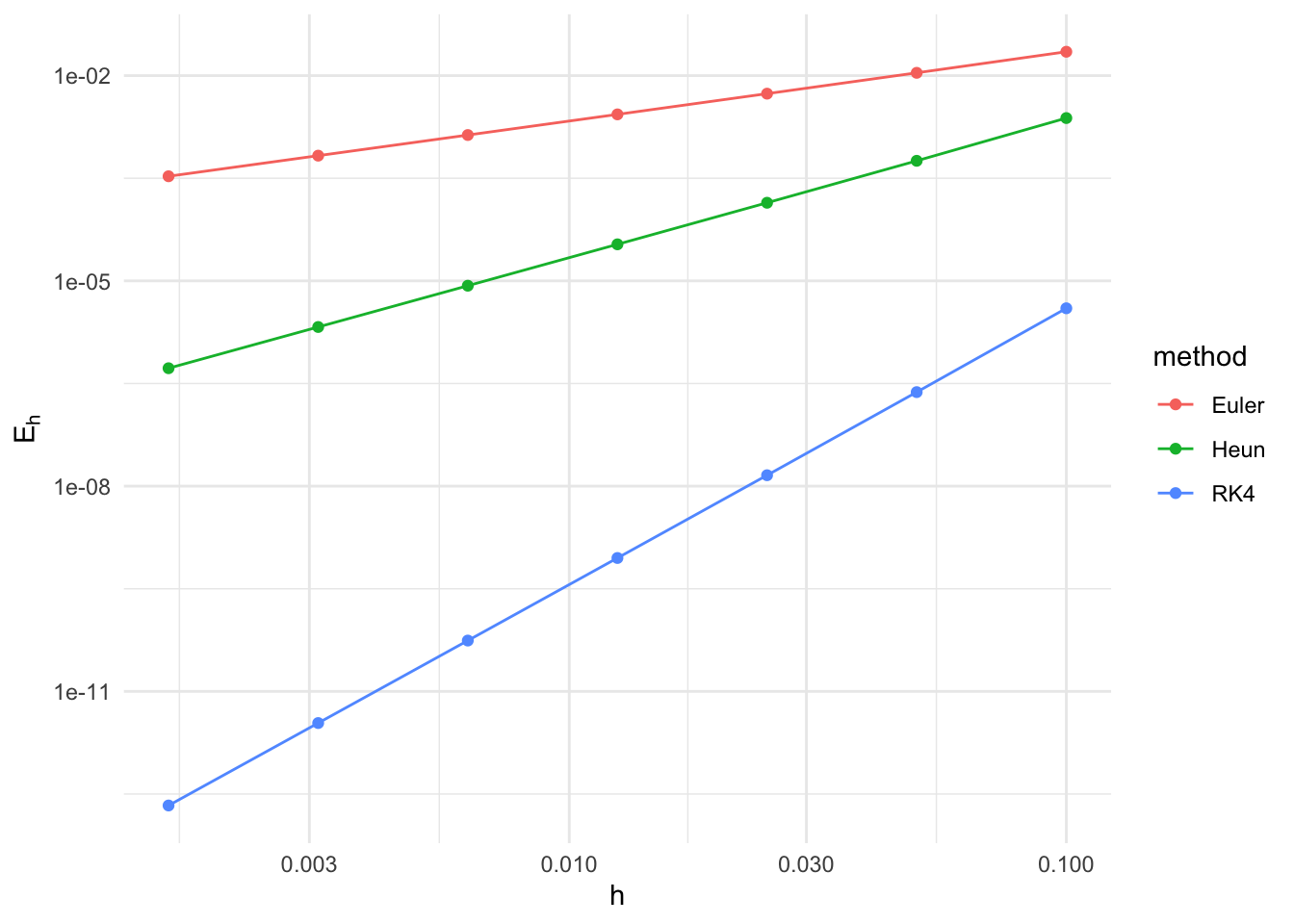
so that plotting \log E_h against \log h gives a straight line of slope p and intercept \log C. Good linearity over several refinements is itself part of the verification: it confirms that the method is in its asymptotic regime.
so that for y_0=\frac14 the exponential term disappears and the solution is the polynomial t(t-1)/2+1/4. The right-hand side still depends on y, so no method below reproduces it exactly — the test is a genuine one. We integrate on [0,1] with the explicit Euler, Heun and classical RK4 methods, halving the step size seven times.
f <-function(y, t) -2* y + t^2exact <-function(t, y0) t * (t -1) /2+1/4+exp(-2* t) * (y0 -1/4)# generic explicit one-step driver: y_{k+1} = y_k + h * Psi(t_k, y_k, h)one_step <-function(Psi, t0, y0, h, t_end) { t <-seq(t0, t_end, by = h) y <-numeric(length(t)); y[1] <- y0for (i inseq_len(length(t) -1)) y[i +1] <- y[i] + h *Psi(t[i], y[i], h)data.frame(t = t, y = y)}psi_euler <-function(t, y, h) f(y, t)psi_heun <-function(t, y, h) { k1 <-f(y, t); k2 <-f(y + h * k1, t + h); (k1 + k2) /2}psi_rk4 <-function(t, y, h) { k1 <-f(y, t); k2 <-f(y + h/2* k1, t + h/2) k3 <-f(y + h/2* k2, t + h/2); k4 <-f(y + h * k3, t + h) (k1 +2*k2 +2*k3 + k4) /6}t0 <-0; y0 <-0.25; t_end <-1hs <-0.1/2^(0:6)max_error <-function(Psi) sapply(hs, function(h) { s <-one_step(Psi, t0, y0, h, t_end)max(abs(s$y -exact(s$t, y0)))})E <-data.frame(h = hs,Euler =max_error(psi_euler),Heun =max_error(psi_heun),RK4 =max_error(psi_rk4))tabE <- EtabE[-1] <-lapply(tabE[-1], formatC, format ="e", digits =2)tabE$h <-formatC(E$h, format ="e", digits =2)knitr::kable(tabE, align ="r",col.names =c("$h$", "Euler", "Heun", "RK4"),caption ="Maximum error $E_h$ on $[0,1]$.")
Maximum error E_h on [0,1].
h
Euler
Heun
RK4
1.00e-01
2.23e-02
2.40e-03
3.98e-06
5.00e-02
1.10e-02
5.69e-04
2.37e-07
2.50e-02
5.45e-03
1.39e-04
1.44e-08
1.25e-02
2.71e-03
3.42e-05
8.91e-10
6.25e-03
1.35e-03
8.50e-06
5.53e-11
3.13e-03
6.76e-04
2.12e-06
3.45e-12
1.56e-03
3.38e-04
5.29e-07
2.15e-13
The observed orders between consecutive refinements follow from Equation 2.2:
The three columns converge to 1, 2 and 4, matching the theoretical orders. A single global estimate can also be obtained by least squares on the log-log data, which is what the slopes of the following plot represent.
Figure 2.1: Maximum error versus step size in logarithmic scale. The slopes are the observed orders.
WarningHow to read an order verification
Look for a plateau, not a single number. Three or four consecutive estimates settling on the same value are evidence; one value is not.
Stay in the useful window. The estimate is meaningful only when h is small enough for the asymptotic regime Equation 2.1 to hold, and large enough that E_h is well above the rounding level \sim\varepsilon_{\rm
mach}. For a fourth-order method on a smooth problem this window can be only two or three refinements wide, which is why the verification should be run with a loose tolerance rather than at the limit of machine precision.
A wrong order is informative. An observed order of 1 for a method designed to be of order 2 usually means a misplaced h in the increment function; an observed order one higher than expected usually means the test problem is too special — a polynomial solution, for instance, can be integrated exactly by a method of sufficient order.
Without an exact solution, replace y(t_k) by a reference computed on a much finer mesh, or use the three-mesh estimator p\approx\log_2\bigl|(y^{4h}-y^{2h})/(y^{2h}-y^{h})\bigr|, which needs no exact solution at all.
Summary
A one-step method is written y_{k+1}=y_k+h\Psi(t_k,y_k;h); the whole theory relates the local defect\mathcal O(h^{p+1}) to the global error\mathcal O(h^{p}).
The convergence theorem Theorem 2.1 gives the explicit bound \frac{C}{L_\Psi}\bigl(e^{L_\Psi(t_k-t_0)}-1\bigr)h^{p}: the Lipschitz property of f is the only substantial hypothesis.
Explicit Euler has order 1; Heun and Collatz reach order 2 with two evaluations of f per step.
Implicit Euler and Crank–Nicolson require solving an equation at every step but have far better stability properties.
The order is verified numerically from the ratio of errors at halved step sizes, Equation 2.2 — a check that should accompany every implementation.