University of Trento, Department of Industrial Engineering
6.1 Why study stability? Start with explicit Euler
Consider the simple initial-value problem
y'(t)=-y(t),\qquad y(0)=1.
Its exact solution is y(t)=e^{-t}: it is positive, decreases monotonically, and tends to zero. With a constant step h>0, explicit Euler gives
y_{n+1}=y_n+h(-y_n)=(1-h)y_n,\qquad y_n=(1-h)^n.
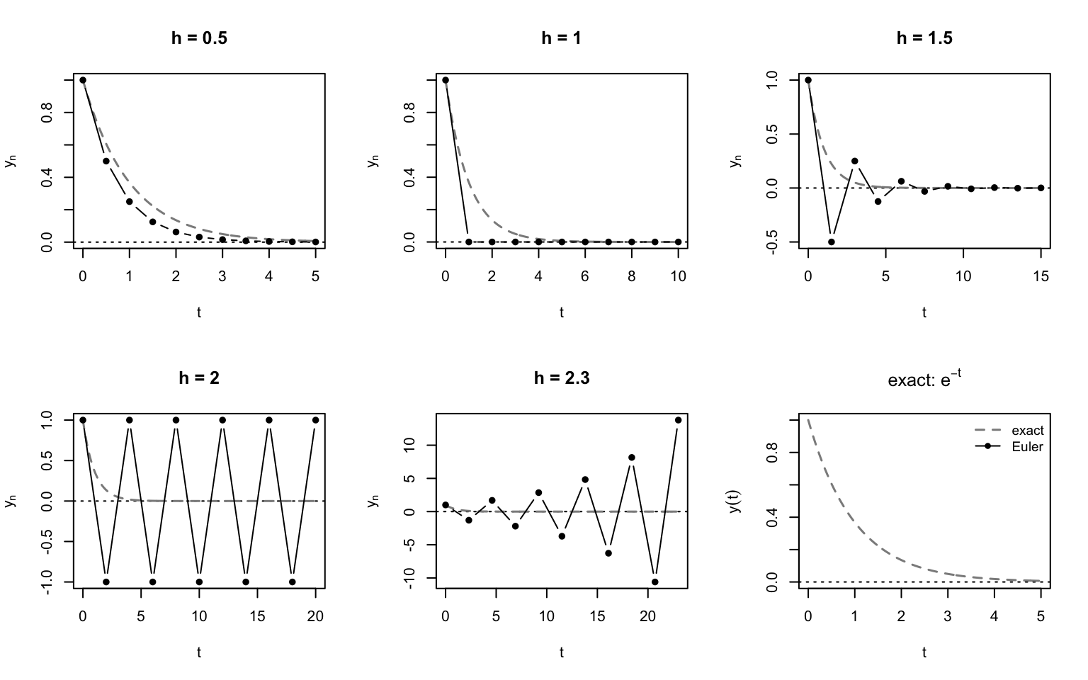
The numerical behavior changes dramatically as h varies:
Step size
Amplification 1-h
Numerical behavior
0<h<1
0<1-h<1
positive monotone decay
h=1
0
reaches zero in one step
1<h<2
-1<1-h<0
alternating signs, decreasing amplitude
h=2
-1
undamped sign alternation
h>2
1-h<-1
alternating signs, growing amplitude
The differential equation is perfectly stable, but the numerical solution can diverge. Stability of the ODE and stability of its discretization are different properties. Notice also that decay of the numerical solution does not imply preservation of positivity or monotonicity.
hs <-c(0.5, 1, 1.5, 2, 2.3)par(mfrow =c(2, 3))for (h in hs) { n <-0:10 tn <- n*h yn <- (1-h)^n tt <-seq(0, max(tn), length.out =400)# la curva esatta va disegnata per prima, cosi' i punti di Euler le stanno sopraplot(tn, yn, type ="n",xlab ="t", ylab =expression(y[n]),main =paste("h =", h))abline(h =0, lty =3)lines(tt, exp(-tt), col ="grey55", lty =2, lwd =1.5)lines(tn, yn, type ="b", pch =16)}# sesto riquadro: la sola soluzione esatta, sullo stesso intervallo del caso h = 0.5t <-seq(0, 5, length.out =400)plot(t, exp(-t), type ="n",xlab ="t", ylab =expression(y(t)), ylim =c(0, 1),main =expression(paste("exact: ", e^-t)))abline(h =0, lty =3)lines(t, exp(-t), col ="grey55", lty =2, lwd =1.5)legend("topright", bty ="n", cex =0.9,legend =c("exact", "Euler"),col =c("grey55", "black"), lty =c(2, 1),pch =c(NA, 16), lwd =c(1.5, 1))par(mfrow =c(1, 1))
Figure 6.1: Explicit Euler for y’=-y: decay, alternating decay, neutral oscillations and instability. The exact solution is overlaid in grey.
6.2 Why do complex numbers appear? Linear systems and diagonalization
The scalar example is not an artificial choice. Consider a linear autonomous system
Diagonalization is useful because it separates a coupled system into independent scalar modes. Each mode is described by the same test equation, with a different eigenvalue. A real matrix can have nonreal eigenvalues, so restricting the test equation to real \lambda would miss oscillatory dynamics.
Thus each continuous mode decays when \operatorname{Re}(\lambda)<0. For a diagonalizable system, all modes decay if all eigenvalues have negative real part. Non-diagonalizable systems require Jordan blocks, but the scalar equation still identifies the basic amplification mechanism; for non-normal matrices, transient growth may occur even when all modes are asymptotically stable.
Explicit Euler applied to the system
Explicit Euler applied directly to the system yields
\bm y_{n+1}=(\bm I+h\bm A)\bm y_n.
In modal coordinates,
z_{j,n+1}=(1+h\lambda_j)z_{j,n}.
The continuous mode decays if \operatorname{Re}(\lambda_j)<0, whereas the discrete mode decays strictly if
\boxed{|1+h\lambda_j|<1.}
For the example \lambda=-1+4i,
|1+h\lambda|^2=(1-h)^2+16h^2=1-2h+17h^2.
Hence explicit Euler damps both oscillatory modes only if 0<h<2/17. The restriction is much more severe than h<2, obtained from the scalar equation y'=-y. This is precisely why stability must be studied in the complex plane.
6.3 The complex scalar test equation and the stability region
The standard Dahlquist test equation is
z'(t)=\lambda z(t),\qquad \lambda\in\mathbb C.
Over one step its exact amplification is
z(t_{n+1})=e^qz(t_n),\qquad q=h\lambda.
For a one-step method, define its stability functionR(q) through
z_{n+1}=R(q)z_n,\qquad z_n=R(q)^nz_0.
For a fixed step, |R(q)|<1 gives asymptotic decay; |R(q)|=1 gives bounded constant-amplitude propagation for this scalar recurrence; |R(q)|>1 gives growth. We distinguish the closed non-amplification region
\boxed{\mathcal S=\{q\in\mathbb C:|R(q)|\le1\}}
from its strict interior |R(q)|<1, which gives decay. Boundary points need care: boundedness does not mean decay. For consistent methods R(q)=1+q+\mathcal O(q^2) near q=0.
Important. Absolute stability of the test equation is distinct from existence and uniqueness of ODE solutions, consistency, zero-stability, convergence and accuracy.
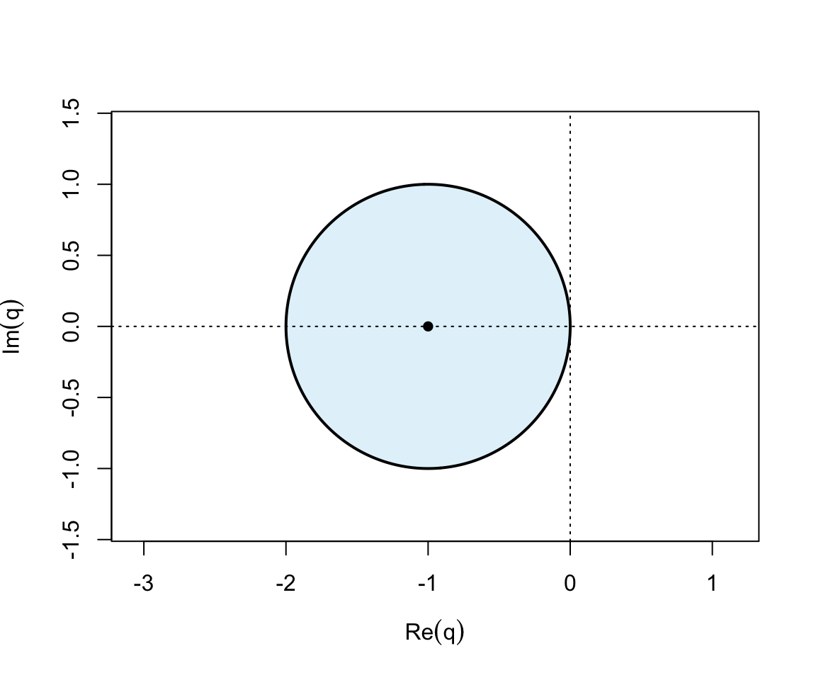
This is the closed disk centered at (-1,0) with radius 1. For strictly decaying modes one needs the open disk. Along the negative real axis the closed interval is [-2,0], and for \lambda<0 the strict-decay condition is 0<h<2/|\lambda|. At h=2/|\lambda| the numerical mode alternates without decay.
th <-seq(0, 2*pi, length.out =500)plot(-1+cos(th), sin(th), type ="l", asp =1,xlim =c(-2.5, 0.6), ylim =c(-1.4, 1.4),xlab =expression(Re(q)), ylab =expression(Im(q)))polygon(-1+cos(th), sin(th), col =adjustcolor("skyblue", alpha.f =0.25), border =NA)lines(-1+cos(th), sin(th), lwd =2)abline(h =0, v =0, lty =3)points(-1, 0, pch =16)
Figure 6.2: Explicit Euler stability disk in the complex q-plane, including its boundary.
For a diagonalizable system, each scaled eigenvalue q_j=h\lambda_j must lie in this disk to prevent growth of its mode. This geometric condition explains the meaning of a stability region: varying h moves every point h\lambda_j along a ray from the origin.
6.4 Runge–Kutta methods: deriving the stability function step by step
We now derive, rather than merely state, the amplification factor of Runge–Kutta methods. We use the scalar test equation
z'=\lambda z,\qquad q=h\lambda,\qquad \lambda\in\mathbb C.
For an s-stage RK method, with Butcher coefficients A=(a_{ij}), b=(b_i) and c=(c_i), define the stage incrementsK_i by
More generally, all explicit two-stage RK methods of order two (including Ralston’s method) have this same stability polynomial, despite having different stage coefficients. On the negative real axis, their closed non-amplification interval is [-2,0]: order two does not, by itself, increase the stable step for a real negative eigenvalue relative to explicit Euler.
This is the degree-four Taylor polynomial of e^q. The closed stability interval along the negative real axis is approximately [-2.785293563,0]. The region is nevertheless bounded, as for every explicit RK method.
General RK stability function from the Butcher tableau
The previous calculations can be collected in matrix notation. Set
For implicit RK methods, A need not be nilpotent and R(q) is generally rational, with poles at zeros of \det(I-qA). Its stability region is the set of points where the function is defined and |R(q)|\le1. This formula also provides a systematic route to stability-region plots for arbitrary Butcher tableaux.
Implicit Euler
Implicit Euler gives
z_{n+1}=z_n+qz_{n+1},
and hence
\boxed{R_{\rm IE}(q)=\frac{1}{1-q}.}
The stability condition is
|1-q|\ge1.
The entire closed left half-plane belongs to \mathcal S, so implicit Euler is A-stable. Moreover,
Thus the trapezoidal rule is not L-stable. Extremely stiff decaying modes are not damped to zero; instead they can survive numerically as alternating oscillations. This is a fundamental practical difference between trapezoidal and implicit Euler.
6.5 A-Stability and L-Stability
Definition 6.1 (Definition: A-Stability) A one-step method is A-stable if
\boxed{
\{q\in\mathbb C:\operatorname{Re}(q)\le0\}\subseteq\mathcal S.
}
Thus every stable mode of the scalar test equation remains numerically stable for every positive step size.
Definition 6.2 (Definition: L-Stability) An A-stable one-step method is L-stable if additionally
\boxed{
R(q)\to0
\quad\text{as }|q|\to\infty
\text{ in the left half-plane}.
}
A-stability prevents growth of arbitrarily stiff stable modes; L-stability additionally suppresses them. This distinction is important for dissipative stiff systems.
6.6 Stability for Systems and Multistep Methods
From the Scalar Test Equation to Systems
Consider the linear system
\bm{y}'=\bm{A}\bm{y}.
For a Runge–Kutta method the scalar stability function extends formally to the matrix argument
\bm{y}_{n+1}=R(h\bm{A})\bm{y}_n.
If \bm{A} is diagonalizable,
\bm{A}=\bm{V}\bm{\Lambda}\bm{V}^{-1},
then
R(h\bm{A})
=\bm{V}R(h\bm{\Lambda})\bm{V}^{-1}.
The eigenvalues h\lambda_j therefore indicate which scalar stability modes are present. A common practical requirement is
h\lambda_j\in\mathcal S
\qquad\text{for all relevant eigenvalues }\lambda_j.
For normal matrices this spectral picture is especially informative. For strongly non-normal matrices, eigenvalues alone can be insufficient because transient growth may be governed by the conditioning of \bm{V}, the pseudospectrum, or related non-normal effects. Absolute-stability plots should therefore not be interpreted as a complete stability theory for every nonlinear or non-normal problem.
Unlike a one-step method, a multistep method generally has several amplification roots \xi_j(q). Therefore stability cannot in general be described by a single function R(q).
Definition 6.3 (Definition: Absolute Stability for an LMM) A value q belongs to the absolute-stability region if every root of
\pi(\xi;q)=0
satisfies
|\xi_j(q)|\le1,
and every root on |\xi|=1 is simple.
The simplicity condition is essential: a repeated unit-modulus root produces polynomial growth in the recurrence even though its modulus is one.
Boundary-Locus Method
At a regular point of the stability boundary, at least one characteristic root lies on the unit circle. Set
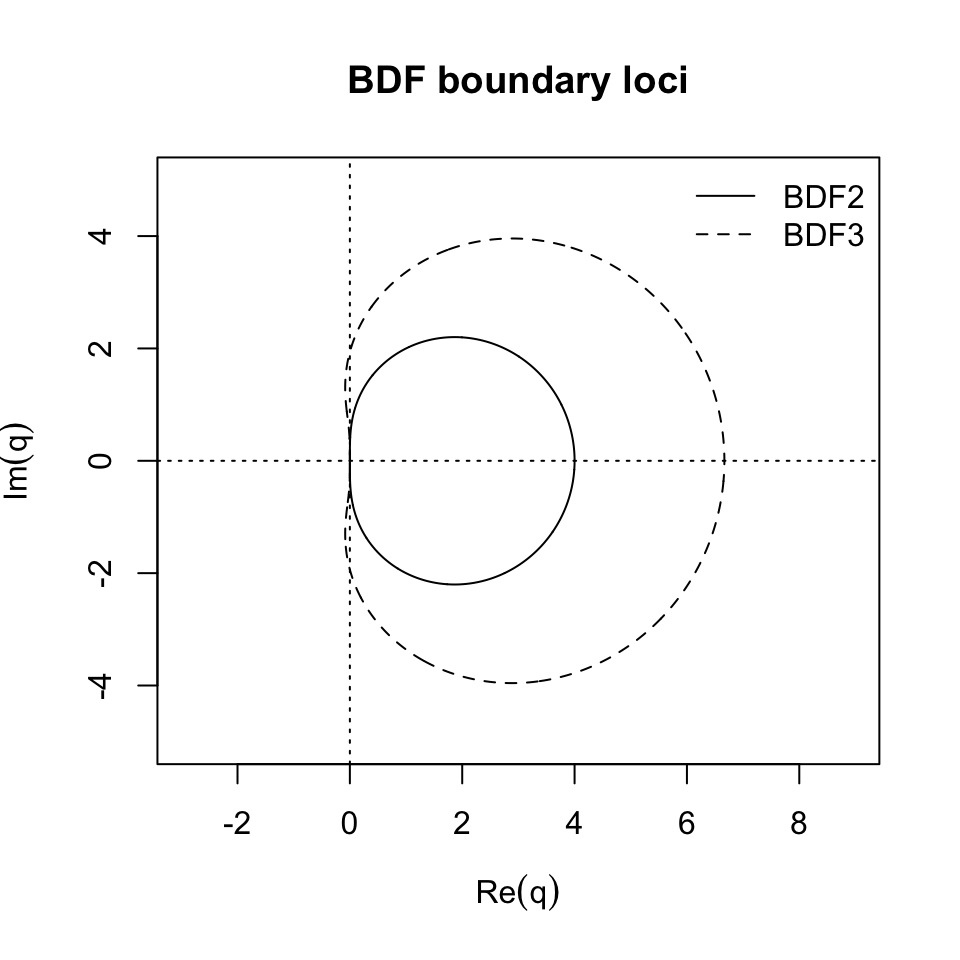
This is the boundary locus. The curve alone does not determine which side is stable; one must test a point in each connected component or directly inspect the roots of \pi(\xi;q).
BDF3 is not A-stable: its region does not contain the entire left half-plane. Nevertheless it is A(\alpha)-stable: a sector
\{q:\ |\arg(-q)|\le\alpha\}
about the negative real axis lies inside the stability region. For BDF3, \alpha\approx86.03^\circ. This explains why higher-order BDF methods remain useful for many stiff dissipative problems despite the second Dahlquist barrier.
6.7 Stability Diagrams and Examples
Stability Plots
The following code generates the stability regions used for comparison. The plots are computed from the defining stability conditions rather than from hard-coded boundary curves.
# L'altezza conta: con asp = 1 R impone la stessa scala sui due assi, quindi# se il riquadro e' piu' alto di quanto serve e' l'asse y a dilatarsi per# riempirlo. A 7x6, con tre riquadri affiancati, y arrivava a +/-10.24# invece dei +/-4 della griglia. A 7x3 viene +/-4.32.R_EE <-function(q) 1+ qR_RK2 <-function(q) 1+ q + q^2/2R_RK4 <-function(q) 1+ q + q^2/2+ q^3/6+ q^4/24x <-seq(-4, 2, length.out =600)y <-seq(-4, 4, length.out =600)q <-outer(x, y, function(a, b) a +1i*b)plot_region <-function(R, main, xlim =range(x), ylim =range(y)) { z <-Mod(R(q))contour(x, y, z, levels =1, drawlabels =FALSE,xlab =expression(Re(q)), ylab =expression(Im(q)),main = main, xlim = xlim, ylim = ylim, asp =1)abline(h =0, v =0, lty =3)}par(mfrow =c(1, 3))plot_region(R_EE, "Explicit Euler")plot_region(R_RK2, "RK2")plot_region(R_RK4, "Classical RK4")par(mfrow =c(1, 1))
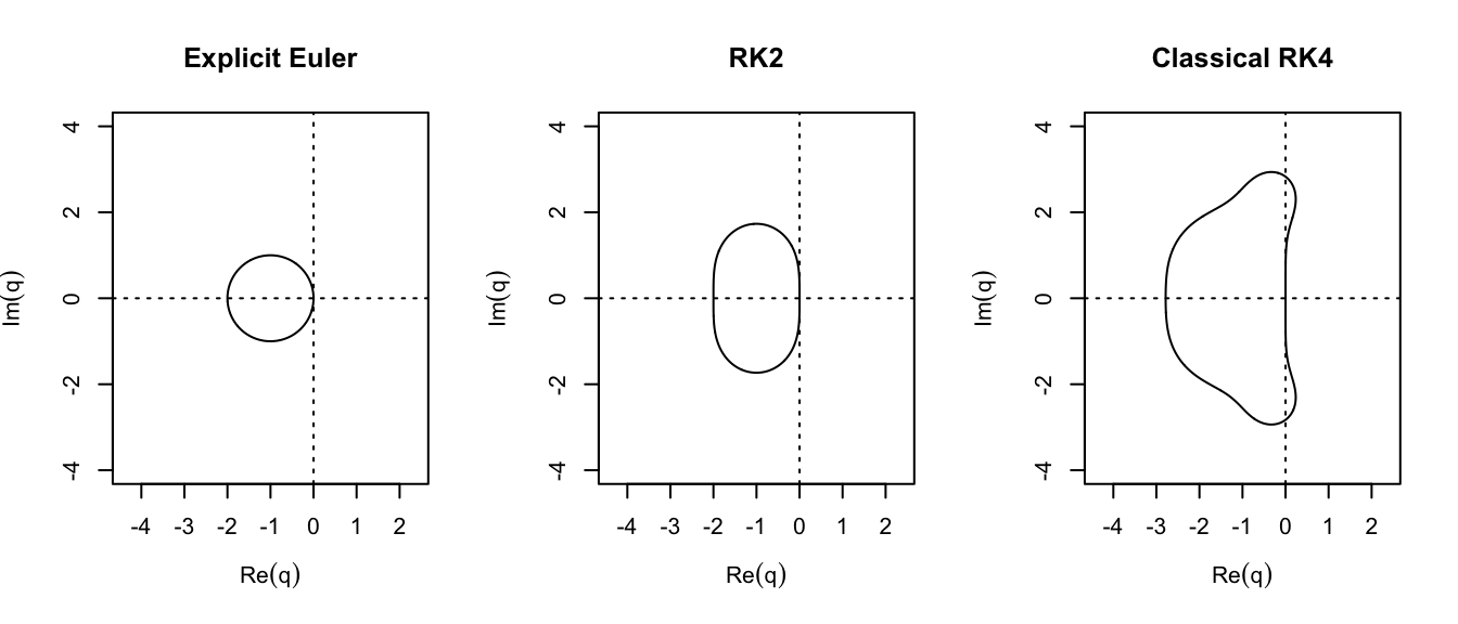
Figure 6.3: Absolute-stability regions of explicit Euler, RK2, and classical RK4.
The bounded regions make the limitation of explicit methods immediately visible. Increasing the order changes the shape and extent of the stability region, but does not produce A-stability.
R_IE <-function(q) 1/(1-q)R_TR <-function(q) (1+q/2)/(1-q/2)x2 <-seq(-8, 4, length.out =700)y2 <-seq(-6, 6, length.out =700)q2 <-outer(x2, y2, function(a, b) a +1i*b)par(mfrow =c(1, 2))contour(x2, y2, Mod(R_IE(q2)), levels =1, drawlabels =FALSE,xlab =expression(Re(q)), ylab =expression(Im(q)),main ="Implicit Euler", asp =1)abline(h =0, v =0, lty =3)contour(x2, y2, Mod(R_TR(q2)), levels =1, drawlabels =FALSE,xlab =expression(Re(q)), ylab =expression(Im(q)),main ="Trapezoidal rule", asp =1)abline(h =0, v =0, lty =3)par(mfrow =c(1, 1))
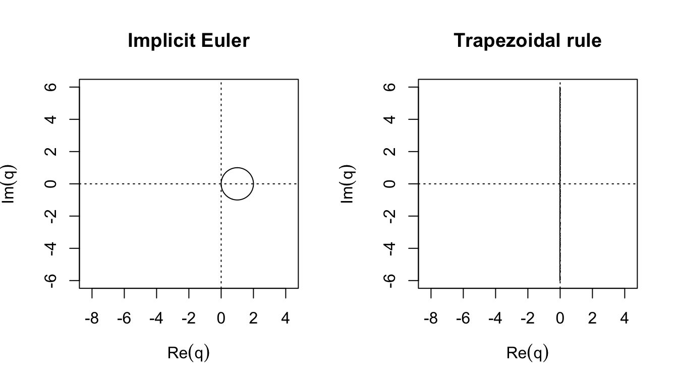
Figure 6.4: Absolute-stability boundaries of implicit Euler and the trapezoidal rule. Both methods contain the left half-plane; only implicit Euler is L-stable.
For implicit Euler the boundary is the circle |1-q|=1, but the stable side is the exterior of that circle. For the trapezoidal rule the boundary is the imaginary axis and the stable side is the entire left half-plane.
Figure 6.5: Boundary loci for BDF2 and BDF3. The stable component is identified using the root condition.
A boundary-locus plot should always be read together with the root condition. In particular, the stability region of BDF methods is the unbounded component on the left side of the relevant boundary, not the bounded area enclosed visually by a curve.
The exact solution contains a slow mode e^{-t} and a fast mode e^{-1000t}. For explicit Euler, stability of the fast mode requires
|-1{,}000h+1|\le1,
hence
\boxed{h\le0.002.}
After the initial transient has decayed, the physically relevant solution may vary on a time scale of order one, yet explicit Euler must continue to take at least 500 steps per unit time solely because of stability.
Implicit Euler has no such stability restriction because every q<0 lies in its stability region. Moreover, its L-stability rapidly removes the -1000 mode. The trapezoidal rule is A-stable but not L-stable; with a very large negative q its amplification factor approaches -1, so the fast mode can appear as a weakly damped numerical oscillation.
This example captures the computational meaning of stiffness: the step size of an explicit method is dictated by stability rather than by the accuracy needed for the solution component of interest.
6.8 Practical Guidance
Stability Versus Accuracy
A value q lying inside \mathcal S only guarantees bounded numerical propagation for the test equation. It does not imply that the approximation is accurate. For example, implicit Euler is stable for arbitrarily large negative q, but
R_{\rm IE}(q)=\frac{1}{1-q}
need not accurately approximate e^q at a coarse step size.
A practical step size must therefore satisfy two distinct requirements:
stability: the relevant scaled eigenvalues h\lambda_j must lie in the method’s stability region;
accuracy: the local/global error must satisfy the requested tolerance.
For non-stiff problems accuracy usually determines h. For stiff problems an explicit method can instead be stability-limited.
Oscillatory Problems and the Imaginary Axis
For nearly conservative problems, eigenvalues may lie close to the imaginary axis. Then the behavior of R(i\omega h) matters. Two errors should be distinguished:
dissipation error:|R(i\omega h)|\ne1;
dispersion or phase error:\arg R(i\omega h)\ne\omega h.
A method can therefore be absolutely stable and still reproduce oscillations poorly. For long-time Hamiltonian or wave-like dynamics, geometric properties such as symplecticity may be more informative than absolute stability alone.
Practical Interpretation of Stability Diagrams
When selecting a method or a step size, the following procedure is useful.
Linearize the ODE locally when appropriate:
\bm{y}'\approx\bm{J}_{\bm{f}}(t,\bm{y})\bm{y}+\cdots.
Estimate the relevant eigenvalues \lambda_j of \bm{J}_{\bm{f}}.
Scale them by the candidate step size: q_j=h\lambda_j.
Check whether the q_j lie in the stability region.
Independently enforce the accuracy tolerance.
For strongly non-normal problems this eigenvalue test is only a first diagnostic, not a complete guarantee.
Comparison of Representative Methods
Method
Order
Type
R(q)
Stability on negative real axis
A-stable
L-stable
Explicit Euler
1
explicit RK
1+q
[-2,0]
no
no
Explicit RK2 (Heun, midpoint, Ralston)
2
explicit RK
1+q+\dfrac{q^2}{2}
[-2,0]
no
no
Classical RK4
4
explicit RK
\sum_{k=0}^{4}\dfrac{q^k}{k!}
approximately [-2.7853,0]
no
no
Implicit Euler
1
implicit RK
\dfrac{1}{1-q}
(-\infty,0]
yes
yes
Trapezoidal rule (Crank–Nicolson)
2
implicit RK
\dfrac{1+q/2}{1-q/2}
(-\infty,0]
yes
no
Implicit midpoint
2
implicit RK
\dfrac{1+q/2}{1-q/2}
(-\infty,0]
yes
no
Gauss–Legendre, s stages
2s
implicit RK
Padé (s,s)
(-\infty,0]
yes
no
Radau IIA, s stages
2s-1
implicit RK
Padé (s-1,s)
(-\infty,0]
yes
yes
BDF2
2
implicit LMM
–
(-\infty,0]
yes
–
BDF3
3
implicit LMM
–
(-\infty,0] and a left sector
no
–
For multistep methods, the one-step definition of L-stability through a scalar function R(q) does not apply directly; their stiff-decay behavior is instead analyzed through the roots of \pi(\xi;q) and related notions.
6.9 Geometric Integration and Invariant Preservation
Absolute stability and local error do not completely describe long-time dynamics. A geometric integrator is designed to preserve a structural property of the differential equation—typically symplectic form, momentum, reversibility, positivity, or a first integral—exactly or with a controlled long-time error.
the exact flow is symplectic. A generic high-order method can give a small short-time error while producing systematic energy drift over a long interval. A symplectic method instead preserves a nearby modified Hamiltonian; its energy error is commonly bounded and oscillatory over long times.
Symplectic Euler and Störmer–Verlet
For a separable Hamiltonian H(\bm q,\bm p)=T(\bm p)+V(\bm q), one version of symplectic Euler is
Its symmetry makes the method time reversible and is central to its favorable long-time behavior.
Constraints and invariants
For holonomic constraints \bm\Phi(\bm q)=\bm0, SHAKE and RATTLE augment a Verlet-type step with Lagrange multipliers so that position constraints, and for RATTLE also velocity constraints, hold at the accepted state. This links geometric ODE integration to the projection and coordinate methods used for DAEs in Section 8.10.
Not every invariant should be enforced by an arbitrary projection. Projection can destroy symplecticity, and exact energy conservation can distort phase. The property to preserve must follow from the qualitative behavior that matters for the model.
A practical long-time test
When comparing methods on a conservative problem, report
state error over a fixed short interval;
energy and momentum errors over a long interval;
constraint residuals when constraints are present;
phase or period error;
the same quantities under step refinement.
This separates high local accuracy from faithful qualitative dynamics.
Summary
Absolute stability explains why methods of the same order can behave very differently on stiff problems. The principal points are:
explicit Runge–Kutta stability regions are bounded;
A-stable methods contain the entire left half-plane;
L-stability adds strong damping of very stiff stable modes;
the trapezoidal rule is A-stable but not L-stable;
BDF2 is A-stable, whereas BDF3–BDF6 retain only sectorial stability;
for multistep methods stability is governed by all characteristic roots;
stability and accuracy are independent requirements;
eigenvalue-based stability diagrams are powerful diagnostics but are not a complete theory for nonlinear or strongly non-normal systems;
geometric structure and invariants can dominate long-time behavior even when classical stability requirements are satisfied.
These ideas connect the qualitative theory of ODEs, the Runge–Kutta framework, and the zero-stability/convergence theory of linear multistep methods developed in the preceding chapters.