
8 Numerical Methods for DAEs
This unit covers consistent initialization, direct and implicit integration, constraint drift, Baumgarte stabilization, projection, coordinate partitioning, order reduction, and method selection. Each topic is a section of this chapter.
8.1 Consistent Initialization
A DAE cannot in general be started from arbitrary values. For the implicit system
\bm F(\bm y,\dot{\bm y},t)=\bm0,
the pair (\bm y_0,\dot{\bm y}_0) is consistent when it satisfies the original equations and every hidden constraint required by the index. An inconsistent start commonly produces a failed Newton iteration, a large initial transient, or constraint drift that is incorrectly attributed to the time integrator.
TipLearning objectives
After this chapter, the reader should be able to identify differential and algebraic unknowns, construct the consistency residual, compute a nearby consistent state, and verify the result before starting time integration.
A practical procedure
For a semi-explicit index-1 problem
\dot{\bm x}=\bm f(\bm x,\bm z,t), \qquad \bm0=\bm g(t,\bm x,\bm z),
the following workflow is robust.
- Choose the fixed data. Decide which components of \bm x_0 are prescribed by the physical experiment and which may be corrected.
- Solve the algebraic equations. With the prescribed components fixed, solve \bm g(t_0,\bm x_0,\bm z_0)=\bm0 for the remaining state and algebraic variables.
- Recover derivatives. Set \dot{\bm x}_0=\bm f(\bm x_0,\bm z_0,t_0).
- Add hidden constraints. For index q>1, differentiate the algebraic constraints only as far as required and append those relations to the nonlinear system. Alternatively, first apply an index-reduction method.
- Scale and solve. Scale every residual by a characteristic magnitude and use a damped Newton or nonlinear least-squares method.
- Verify independently. Report the norm of the original DAE residual, every hidden-constraint residual, and the size of the correction to the user-supplied data.
This order matters: merely satisfying the visible algebraic constraint does not guarantee that the derivative lies in its tangent space.
Projection to nearby consistent data
Suppose an approximate state \widetilde{\bm y}_0 is available and the assembled consistency conditions are \bm c(\bm y_0)=\bm0. A nearby consistent state can be defined by
\min_{\bm y_0}\ \frac12 \|\bm W(\bm y_0-\widetilde{\bm y}_0)\|_2^2 \quad\text{subject to}\quad \bm c(\bm y_0)=\bm0, \tag{8.1}
where \bm W protects accurately known components and accounts for units. One Newton–KKT correction solves
\begin{bmatrix} \bm W^T\bm W & \bm C^T\\ \bm C & \bm0 \end{bmatrix} \begin{bmatrix}\Delta\bm y\\\Delta\bm\lambda\end{bmatrix} =- \begin{bmatrix} \bm W^T\bm W(\bm y-\widetilde{\bm y}_0)+\bm C^T\bm\lambda\\ \bm c(\bm y) \end{bmatrix},
with \bm C=\partial\bm c/\partial\bm y. Rank deficiency of \bm C is a model diagnostic: redundant constraints should be removed or treated with a rank-revealing factorization.
Acceptance checklist
A computed initialization is acceptable only if
- scaled DAE and hidden-constraint residuals meet the requested tolerance;
- the constraint Jacobian has the expected numerical rank;
- the correction in Equation 8.1 is physically reasonable;
- one trial implicit step converges without an anomalous reduction of the step size.
The case studies in the companion volume (Case Studies) show how these checks change for mechanical, circuit, and high-index models.
8.2 Implicit Integration of Linear DAEs
Consider the DAE
\begin{aligned} x(t) &=\sin(t) \\ x'(t)+y(t) &= 0 \end{aligned}
with exact solution
\begin{aligned} x(t) &= \sin(t) \\ y(t) &= -\cos(t) \end{aligned}
Is a linear DAE \bm{F}\bm{x}'(t)+\bm{G}\bm{x}(t)=\bm{h}(t) where
\begin{pmatrix} 0 & 0 \\ 1 & 0 \end{pmatrix} \begin{pmatrix} x' \\ y' \end{pmatrix}+ \begin{pmatrix} 1 & 0 \\ 0 & 1 \end{pmatrix} \begin{pmatrix} x \\ y \end{pmatrix}= \begin{pmatrix} \sin(t) \\ 0 \end{pmatrix}
Using Kronecker/Weierstrass normal form with
\bm{U}=\bm{V}=\begin{pmatrix} 0 & 1 \\ 1 & 0 \end{pmatrix} \qquad\text{and}\qquad \bm{N}=\begin{pmatrix} 0 & 1 \\ 0 & 0 \end{pmatrix}
the DAE is written as
\bm{N} \begin{pmatrix} y' \\ x' \end{pmatrix}+ \bm{I} \begin{pmatrix} y \\ x \end{pmatrix}= \begin{pmatrix} 0 \\ \sin(t) \end{pmatrix}
because \bm{N}\neq\bm{0} and \bm{N}^2=\bm{0} the DAE is of index 2. No initial conditions are required because block \bm{C} is absent.
Consistent Initial Values
Reconsider
\begin{aligned} x(t) &=\sin(t) \\ x'(t)+y(t) &= 0 \end{aligned}
I initial values x_0 and y_0 are consistent if
x(t) =\sin(t)
the hidden constraint is obtained by deriving the algebraic part
-y(t) = x'(t) = \cos(t)
and thus consistent initial condition must satisfy:
\begin{aligned} x_0 &=\sin(0) \\ y_0 &=-\cos(0) \end{aligned}
Explicit Euler
Consider the ODE \bm{x}'=\bm{f}(\bm{x},t), explicit Euler take the form
\bm{x}_{k+1} = \bm{x}_k + h \bm{f}(\bm{x}_k,t_k)
applied to the DAE become (t_k=kh)
\begin{aligned} 0 &= h(\sin(t_k) -x_k) \\ x_{k+1} &= x_k - h y_k \end{aligned}
Thus, the method cant be applied (y_{k+1} do not appear in the equations).
Implicit Euler
For \bm{x}'=\bm{f}(\bm{x},t), implicit Euler take the form
\bm{x}_{k+1} - h \bm{f}(\bm{x}_{k+1},t_{k+1}) = \bm{x}_k
Applied to the DAE result in (t_k=k\,h)
\begin{aligned} h(\sin(t_{k+1}) -x_{k+1}) &= 0 \\ x_{k+1} + h y_{k+1} &= x_k \end{aligned}
so that
\begin{aligned} x_{k+1} &= \sin(t_{k+1}) \\ y_{k+1} &= (x_k - \sin(t_{k+1})/h \\ &= (\sin(t_k) - \sin(t_{k+1}))/h =\color{red} -\cos(t_{k+1}) + \mathcal{O}(h) \end{aligned}
Implicit Euler Results
Crank-Nicolson
\frac{\bm{x}_{k+1}-\bm{x}_k}{h} = \frac{\bm{f}(\bm{x}_{k+1},t_{k+1})+\bm{f}(\bm{x}_k,t_k)}{2}
Applied to the DAE result in
\begin{aligned} \sin(t_{k+1}) -x_{k+1} &= x_k - \sin(t_k) \\ x_{k+1} - \frac{h}{2} y_{k+1} &= x_k + \frac{h}{2} y_{k} \end{aligned}
so that
\begin{aligned} x_{k+1} &= \sin(t_{k+1})+\sin(t_k)-x_k \\ y_{k+1} &= \frac{2}{h}(x_{k} - x_{k+1}) - y_k \end{aligned}
solving for x_k
x_k = \sin(t_k)+(-1)^k x_0
Baumgarte Stabilization
Re-consider the DAE
\begin{aligned} x(t) &= \sin(t) \\ x'(t)+y(t) &= 0 \end{aligned}
stabilize the constraint x(t)-\sin(t)=0 using Baumgarte
\begin{aligned} \tau (x(t)-\sin(t))' + (x(t)-\sin(t)) &= 0 \\ x'(t)+y(t) &= 0 \end{aligned}
TipObservation
The ODE \tau z'(t) + z(t) = 0 has solution
z(t) = z(0)\exp\bigg(-\frac{t}{\tau}\bigg) and \lim_{t\to\infty}z(t)=0
Using Crank-Nicolson
\begin{aligned} \frac{\tau}{h}(x_{k+1}-x_k)- \frac{\tau}{h}(\sin(t_{k+1})-\sin(t_k)) &+ \\[0.25em] \frac{1}{2}(x_{k+1}+x_k)- \frac{1}{2}(\sin(t_{k+1})+\sin(t_k)) &= 0 \\[0.25em] \frac{x_{k+1}-x_k}{h}+\frac{y_{k+1}+y_k}{2} &= 0 \end{aligned}
solving for x_{k+1} and y_{k+1}
\begin{aligned} x_{k+1}&=\frac{2\,\tau-h}{2\,\tau+h}\big(x_k-\sin(t_k)\big)+\sin(t_{k+1}) \\[0.25em] y_{k+1}&=\frac{ \sin(t_k)(4\tau-2h)-\sin(t_{k+1})(4\tau+2h)+4hx_k}{h(2\tau+h)} -y_k \end{aligned}
Crank–Nicolson Results
Implicit Eulero seems to work also with inconsistent data.
Crank-Nicolson do not work with inconsistent data
Baumgarte stabilization work well but there is no general recipt to determine stabilization parameters (\tau in this case).
8.3 Constraint Drift
Index reduction replaces some algebraic constraints by their time derivatives. The continuous solution still satisfies the original constraints, but a numerical trajectory generally does not. The resulting departure from the constraint manifold is called constraint drift.
For a holonomic mechanical constraint \bm\Phi(\bm q,t)=\bm0, define
\bm r_p=\bm\Phi(\bm q,t), \qquad \bm r_v=\bm\Phi_{\bm q}\dot{\bm q}+\bm\Phi_t.
An acceleration-level formulation enforces \dot{\bm r}_v=\bm0, not necessarily \bm r_p=\bm0 or \bm r_v=\bm0. Local truncation and nonlinear solver errors therefore act as forcing terms in the residual dynamics.
Why drift accumulates
If the numerical acceleration satisfies
\dot{\bm r}_v=\bm\delta(t),
then
\bm r_v(t)=\bm r_v(t_0)+\int_{t_0}^t\bm\delta(s)\,\mathrm ds,
and the position residual contains a second integration of the defect. Even small, nearly unbiased errors can therefore generate visible long-time drift. Reducing the step size may delay the effect but does not change this neutral residual dynamics.
What to monitor
Report at least four histories:
| Quantity | Diagnostic role |
|---|---|
| \|\bm r_p\| | position-level feasibility |
| \|\bm r_v\| | tangency of the velocity |
| DAE residual | accuracy of the discrete nonlinear solve |
| energy or another invariant | distortion of the physical dynamics |
These quantities distinguish drift from a loose Newton tolerance or an unstable time step.
Remedies
- Baumgarte stabilization assigns asymptotically stable dynamics to the residual; see Section 8.4.
- Projection returns the numerical state to the constraint manifold after a step; see Section 8.5.
- Coordinate partitioning removes redundant coordinates locally; see
- Constraint-preserving integrators enforce the geometry inside the step and are especially attractive for long-time mechanical simulation.
The correct choice depends on index, stiffness, time horizon, and whether exact constraint satisfaction or faithful invariant behavior is the main priority.
8.4 Baumgarte Stabilization
DAEs in Mechanics
This document offers an in-depth exploration of how Differential-Algebraic Equations (DAEs) are formulated and numerically solved, particularly within the context of mechanical systems. It emphasizes systems that involve constraints, which commonly appear in areas like multibody dynamics, robotics, and structural mechanics.
Notation
Consider a mechanical system with the following quantities:
- Generalized (position) coordinates: \bm{p} \in \mathbb{R}^n, representing the configuration of the system.
- Kinetic energy: T(\bm{p}, \bm{p}^{\prime}, t), where \bm{p}^{\prime} is the time derivative of \bm{p}.
- Potential energy: V(\bm{p}, t).
- External generalized forces: \bm{Q}_{ex}(\bm{p}, t) \in \mathbb{R}^n.
- Constraint equations: \bm{\Phi}(\bm{p}, t) \in \mathbb{R}^m, which enforce m constraints on the system.
- Lagrangian:
L(\bm{p}, \bm{p}^{\prime}, t) = T(\bm{p}, \bm{p}^{\prime}, t) - V(\bm{p}, t).
The equations of motion are derived from Lagrange’s equations with constraints:
\frac{\mathrm{d}}{\mathrm{d}t} \left( \frac{\partial L}{\partial \bm{p}^{\prime}} \right) - \frac{\partial L}{\partial \bm{p}} + \left( \frac{\partial \bm{\Phi}(\bm{p}, t)}{\partial \bm{p}} \right)^T \bm{\lambda} = \bm{Q}_{ex}(\bm{p}, \bm{p}^{\prime},t),
where \bm{\lambda} \in \mathbb{R}^m are the Lagrange multipliers enforcing the constraints.
DAE Formulation
Kinetic Energy and Mass Matrix
The kinetic energy is often expressed in terms of the mass matrix \bm{M}(\bm{p},\bm{p}',t):
T(\bm{p}, \bm{p}^{\prime}, t) = \frac{1}{2} (\bm{p}^{\prime})^T \bm{M}(\bm{p},\bm{p}',t) \bm{p}^{\prime}.
Substituting this into the equations of motion yields:
\bm{M}(\bm{p},\bm{p}^{\prime},t) \bm{p}^{\prime\prime} + \left( \frac{\partial \bm{\Phi}}{\partial \bm{p}} \right)^T \bm{\lambda} = \bm{Q}(\bm{p}, \bm{p}^{\prime}, t),
where \bm{Q}(\bm{p}, \bm{p}^{\prime}, t) includes external forces, potential energy gradients, and inertial terms.
Constraint Equations
The constraints \bm{\Phi}(\bm{p}, t) = 0 must be satisfied at all times. Combining these with the equations of motion, we obtain the full DAE system:
\left\{ \begin{aligned} \bm{M}(\bm{p},\bm{p}^\prime t) \bm{p}^{\prime\prime} + \bm{\Phi}_{\bm{p}}(\bm{p}, t)^T \bm{\lambda} &= \bm{Q}(\bm{p}, \bm{p}^{\prime}, t), \\[0.5em] \bm{\Phi}(\bm{p}, t) &= \bm{0}. \end{aligned} \right.
This system has n + m equations and n + m unknowns (\bm{p}^{\prime\prime} and \bm{\lambda}), making it well-posed.
Numerical Scheme
Solving DAEs requires specialized numerical methods due to the presence of algebraic constraints. Below, we outline a common approach based on time discretization and constraint differentiation.
Time Discretization
A simple numerical scheme can be derived using a Taylor expansion in time:
\begin{aligned} \bm{p}^{\prime}(t+\Delta t) &= \bm{p}^{\prime}(t) + \bm{p}^{\prime\prime}(t) \Delta t + \mathcal{O}(\Delta t^2), \\[0.25em] \bm{p}(t+\Delta t) &= \bm{p}(t) + \bm{p}^{\prime}(t) \Delta t + \frac{1}{2} \bm{p}^{\prime\prime}(t) \Delta t^2 + \mathcal{O}(\Delta t^3). \end{aligned}
Neglecting higher-order terms, the updates for position and velocity become:
\begin{aligned} \bm{p}^{\prime}_{k+1} &= \bm{p}^{\prime}_k + {\color{red} \bm{p}^{\prime\prime}_k} \Delta t, \\[0.5em] \bm{p}_{k+1} &= \bm{p}_k + \bm{p}^{\prime}_k \Delta t + \frac{1}{2} {\color{red} \bm{p}^{\prime\prime}_k} \Delta t^2. \end{aligned}
This requires computing \color{red}\bm{p}^{\prime\prime}_k, which involves solving for \bm{\lambda}.
Accelerations and Multipliers
If the mass matrix \bm{M}(\bm{p},\bm{q}^\prime,t) is nonsingular, we can express \bm{p}^{\prime\prime} as:
\bm{p}^{\prime\prime} = \bm{M}(\bm{p},\bm{q}^\prime, t)^{-1} \left[ \bm{Q}(\bm{p}, \bm{p}^{\prime}, t) - \bm{\Phi}_{\bm{p}}(\bm{p}, t)^T \bm{\lambda} \right].
However, \bm{\lambda} is still unknown. To resolve this, we differentiate the constraint equations to incorporate \bm{p}^{\prime\prime}.
Differentiating Constraints
Differentiating the constraints \bm{\Phi}(\bm{p}, t) = \bm{0} once with respect to time yields:
\frac{\mathrm{d}}{\mathrm{d}t} \bm{\Phi}(\bm{p}, t) = \bm{\Phi}_{t} + \bm{\Phi}_{\bm{p}} \bm{p}^{\prime} = \bm{0}.
Differentiating a second time gives:
\bm{\Phi}_{tt} + 2 \bm{\Phi}_{t \bm{p}} \bm{p}^{\prime} + \bm{\Phi}_{\bm{p} \bm{p}} (\bm{p}^{\prime}, \bm{p}^{\prime}) + \bm{\Phi}_{\bm{p}} \bm{p}^{\prime\prime} = \bm{0}.
Rewriting in matrix form:
\begin{pmatrix} \bm{M}(\bm{p},\bm{q}^\prime,t) & \bm{\Phi}_{\bm{p}}^T \\ \bm{\Phi}_{\bm{p}} & \bm{0} \end{pmatrix} \begin{pmatrix} \bm{p}^{\prime\prime} \\ \bm{\lambda} \end{pmatrix} = \begin{pmatrix} \bm{Q}(\bm{p}, \bm{p}^{\prime}, t) \\ \bm{c}(\bm{p}, \bm{p}^{\prime}, t) \end{pmatrix},
where:
\bm{c}(\bm{p}, \bm{p}^{\prime}, t) = -\bm{\Phi}_{tt} - 2\bm{\Phi}_{t \bm{p}} \bm{p}^{\prime} - (\bm{p}^{\prime})^T \bm{\Phi}_{\bm{p} \bm{p}} \bm{p}^{\prime}.
This system can be solved for \bm{p}^{\prime\prime} and \bm{\lambda}.
Integration Algorithm
Initialization
Given initial values t_0 = 0, \bm{p}_0, and \bm{p}^{\prime}_0.
Time Stepping
For each time step k = 0, 1, \dots:
Solve for \bm{p}_k^{\prime\prime} and \bm{\lambda}_k:
\begin{pmatrix} \bm{M}(\bm{p}_k,\bm{p}^\prime_k,t_k) & \bm{\Phi}_{\bm{p}}(\bm{p}_k, t_k)^T \\ \bm{\Phi}_{\bm{p}}(\bm{p}_k, t_k) & \bm{0} \end{pmatrix} \begin{pmatrix} \bm{p}_k^{\prime\prime} \\ \bm{\lambda}_k \end{pmatrix} = \begin{pmatrix} \bm{Q}(\bm{p}_k, \bm{p}_k^{\prime}, t_k) \\ \bm{c}(\bm{p}_k, \bm{p}_k^{\prime}, t_k) \end{pmatrix}.
Update position and velocity:
\begin{aligned} \bm{p}_{k+1}^{\prime} &= \bm{p}_k^{\prime} + \Delta t\,\bm{p}_k^{\prime\prime} \\[0.5em] \bm{p}_{k+1} & = \bm{p}_k + \Delta t\,\bm{p}_k^{\prime} + \frac{1}{2}\Delta t^2 \bm{p}_k^{\prime\prime} . \end{aligned}
Constraint Drift
Over time, numerical errors can cause the system to drift away from the constraints \bm{\Phi}(\bm{p}, t) = \bm{0}. To mitigate this, we redefine the constraints as:
\widetilde{\bm{\Phi}}(\bm{p}, t) = \bm{\Phi}(\bm{p}, t) + \bm{a}_0 + \bm{a}_1 t,
where \bm{a}_0 and \bm{a}_1 are chosen to satisfy the initial conditions:
\widetilde{\bm{\Phi}}(\bm{p}(0),0) = \bm{0}, \quad \frac{\mathrm{d}}{\mathrm{d}t} \widetilde{\bm{\Phi}}(\bm{p}(0),0) = \bm{0}.
If \bm{a}_0 = \bm{a}_1 = \bm{0}, the constraints are perfectly satisfied initially. However, small errors can accumulate, leading to drift over long simulations.
Redundant-Coordinate Pendulum
This section demonstrates the application of Differential-Algebraic Equations (DAEs) to model a pendulum using redundant coordinates. The pendulum is a classic example of a mechanical system with constraints, making it an ideal case study for DAE formulation and numerical solution.
Model
Kinetic and Potential Energy
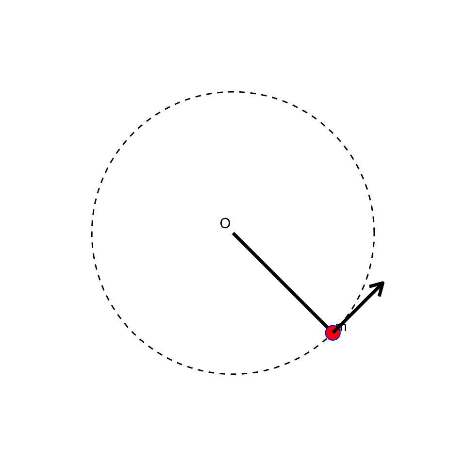
The pendulum consists of a mass m attached to a rigid, massless rod of length 1. The system is described using Cartesian coordinates (x, y), where x and y represent the horizontal and vertical positions of the mass, respectively.
Kinetic energy: T(t) = \frac{1}{2}m \left( x'(t)^2 + y'(t)^2 \right).
Potential energy: V(t) = m g y(t), where g is the gravitational acceleration.
Constraint Equation
The pendulum is constrained to move along a circular path of radius 1. This constraint is expressed as: \Phi(x, y) = x^2 + y^2 - 1 = 0.
Schematic
Equations of Motion
Using Lagrange’s equations with constraints, the equations of motion for the pendulum are:
\left\{ \begin{aligned} m x''(t) + 2x(t)\lambda(t) &= 0, \\[0.5em] m y''(t) + 2y(t)\lambda(t) &= -m g, \\[0.5em] x(t)^2 + y(t)^2 &= 1, \end{aligned} \right. \tag{8.2}
where \lambda(t) is the Lagrange multiplier enforcing the constraint.
Unstabilized Solution
To solve the system numerically Equation 8.2, we differentiate the constraint equation twice to incorporate the acceleration terms x''(t) and y''(t).
First Constraint Derivative
Differentiating \Phi(x, y) = 0 once with respect to time yields: 2x(t)x'(t) + 2y(t)y'(t) = 0.
Second Constraint Derivative
Differentiating again gives: 2x(t)x''(t) + 2y(t)y''(t) + 2x'(t)^2 + 2y'(t)^2 = 0.
This equation introduces the acceleration terms x''(t) and y''(t), allowing us to solve for \lambda(t).
The system of equations can be written in matrix form as:
\begin{pmatrix} m & 0 & 2x(t) \\ 0 & m & 2y(t) \\ 2x(t) & 2y(t) & 0 \end{pmatrix} \begin{pmatrix} x''(t) \\ y''(t) \\ \lambda(t) \end{pmatrix} = \begin{pmatrix} 0 \\ -mg \\ -2x'(t)^2 - 2y'(t)^2 \end{pmatrix}.
Time Discretization
Given initial conditions x_0, y_0, x'_0, and y'_0, we solve the system iteratively using the following steps:
Solve for x''_k, y''_k, and \lambda_k: \begin{pmatrix} m & 0 & 2x_k \\ 0 & m & 2y_k \\ 2x_k & 2y_k & 0 \end{pmatrix} \begin{pmatrix} \color{red} x''_k \\ \color{red} y''_k \\ \color{red} \lambda_k \end{pmatrix} = \begin{pmatrix} 0 \\ -mg \\ -2(x'_k)^2 - 2(y'_k)^2 \end{pmatrix}.
Update position and velocity: \begin{aligned} x_{k+1} &= x_k + \Delta t \, x'_k + \frac{\Delta t^2}{2} \color{red} x''_k, \\ y_{k+1} &= y_k + \Delta t \, y'_k + \frac{\Delta t^2}{2} \color{red} y''_k, \\ x'_{k+1} &= x'_k + \Delta t \, \color{red} x''_k, \\ y'_{k+1} &= y'_k + \Delta t \, \color{red} y''_k. \end{aligned}
Numerical solution shows that the numerical method do not work well
Baumgarte Method
A very popular way to stabilize the constraint \bm{\phi}(\bm{p},t)=0 and thus avoid the drift effect is using Baumgarte’s stabilization, see @baumgarte1972stabilization. This idea is well presented with other techniques in the survey paper @ascher1995stabilization. The key idea is to substitute the constraint with a differential equation that asymptotically satisfies \bm{\phi}(\bm{p},t)=0. Obviously this technique is effective only if you are interested in the long term behaviour, since during transients the constraint may be violated. Since constrained mechanical systems require to differentiations to eliminate the Lagrange multipliers, we consider a linear second order stable differential equation of the form,
\frac{\mathrm{d}^2 z(t)}{\mathrm{d} t^2} + 2\xi\omega_{\textnormal{n}}\frac{\mathrm{d} z(t)}{\mathrm{d} t} + \omega_{\textnormal{n}}^2z(t) = 0, \tag{8.3}
where z(t)\in\mathbb{R}. In this form we recognize the well known equation for second order linear mechanical or electrical systems, such as the RLC circuit or the mass spring damper. In these framework \xi\in\mathbb{R}_{>0} is the damping ratio and \omega_{\textnormal{n}}\in\mathbb{R}_{>0} is the natural frequency. Depending on the value of \xi different cases can arise:
- 0<\xi<1: solution z is underdamped,
- \xi=1: solution z is critically damped,
- \xi>1: solution z is overdamped.
The general form for the solution is the following
z(t) = k_{1}e^{\left(-\xi+\sqrt{\xi^2-1}\right)\omega_{\text{n}}t} + k_{2}e^{\left(-\xi-\sqrt{\xi^2-1}\right)\omega_{\text{n}}t},
where k_{1},k_{2}\in\mathbb{R} are constants determined by the initial conditions z_{0} = z(t=0) and \dot{z}_{0} = \dot{z}(t=0). Solutions for the different cases can be arranged in different ways, here we show some of them. For a deeper treatment see for example @rao1995mechanical. Let us start from the underdamped case; solution takes the form
z(t) = c_ {1}e^{-\xi\omega_{\textnormal{n}}t} \cos\left({\sqrt{1-\xi^2}\omega_{\textnormal{n}}t-c_{2}}\right), \tag{8.4}
where constants c_{1},c_{2}\in\mathbb{R} are given by,
\begin{aligned} c_{1} &= \frac{\sqrt{z_{0}^2 \omega_{\textnormal{n}}^2+\dot{z}_{0}^2+2z_{0}\dot{z}_{0}\xi \omega_{\textnormal{n}}}}{\sqrt{1-\xi^2}\omega_{\textnormal{n}}} \\ c_{2} &= \mathrm{arctan}\left(\frac{\dot{z}_{0}+\xi\omega_{\textnormal{n}}z_{0}} { x_ {0}\omega_{\textnormal{n}}\sqrt{1-\xi^2}}\right). \end{aligned}
As we can observe in Equation 8.4 solution is a cosine function modulated by a decreasing exponential function. For the critically damped case a linear term appears and the solution takes the form,
z(t) = (c_{1}+c_{2}t)e^{-\omega_{\textnormal{n}}t}, \tag{8.5}
where c_{1},c_{2}\in\mathbb{R} are given by c_{1} = z_{0} and c_{2} = \dot{z}_{0}+\omega_{\textnormal{n}}z_{0}. Finally for the overdamped case the solution takes the form
z(t) = c_{1}e^{\left(-\xi+\sqrt{\xi^2-1}\right)\omega_{\textnormal{n}}t} + c_{2}e^{\left(-\xi-\sqrt{\xi^2-1}\right)\omega_{\textnormal{n}}t}, \tag{8.6}
with constants,
\begin{aligned} c_{1} &= \frac{x_{0}\omega_{\textnormal{n}} \left(\xi+\sqrt{\xi^2-1}\right)+\dot{x}_{0}}{2\omega_{\textnormal{n}}\sqrt{\xi^2-1}}, \\ c_{2} &= \frac{-x_{0}\omega_{\textnormal{n}} \left(\xi-\sqrt{\xi^2-1}\right)-\dot{x}_{0}}{2\omega_{\textnormal{n}}\sqrt{\xi^2-1}}. \end{aligned}
However, regardless of the specific form of the solution, all the three cases satisfy a global exponential stability property, i.e., \forall(z_{0},\dot{z}_{0})\in\mathbb{R}\times\mathbb{R} the solution z(t,z_{0},\dot{z}_{0}) satisfies
\lim_{t\rightarrow\infty} z(t,z_{0},\dot{z}_{0}) = 0.
The notation z(t,z_{0},\dot{z}_{0}) is just to stress that the solution depends on time but also from initial conditions (z_{0},\dot{z}_{0}). This consideration suggests to substitute the constraint \bm{\phi}(\bm{p},t) with an ODE of the form Equation 8.3. In this way, despite the initial conditions, the solution will asymptotically satisfies \bm{\phi}(\bm{p},t)=0. Thus the explicit Baumgarte’s stabilization for DAEs of index three takes the form,
\frac{\mathrm{d}^2\bm{\phi}}{\mathrm{d} t^2} + 2\xi\omega_{\textnormal{n}}\frac{\mathrm{d}\bm{\phi}}{\mathrm{d} t} + \omega_{\textnormal{n}}^2\bm{\phi} = 0.
Computing explicitly the terms for mechanical systems the stabilization results,
\frac{\mathrm{d}}{\mathrm{d} t}\frac{\partial\bm{\phi}} {\partial\bm{p}}\dot{\bm{p}}+\frac{\partial\bm{\phi}} {\partial\bm{p}}\ddot{\bm{p}}+\frac{\partial^{2}\bm{\phi}} {\partial t^2} + 2\xi\omega_{\textnormal{n}} \frac{\partial\phi}{\partial\bm{p}}\dot{\bm{p}} + 2\xi\omega_{\textnormal{n}}\frac{\partial\bm{\phi}}{\partial t}+\omega_{\textnormal{n}}^2\bm{\phi} = 0.
which can be re-arranged in the following form
\begin{aligned} -\frac{\partial\bm{\phi}}{\partial\bm{p}}\dot{\bm{v}} & = \frac{\mathrm{d}}{\mathrm{d} t}\frac{\partial\bm{\phi}}{\partial\bm{p}}\bm{v} +\frac{\partial^{2}\bm{\phi}}{\partial t^2} + 2\xi\omega_{\textnormal{n}}\frac{\partial\phi}{\partial\bm{p}}\bm{v} + 2\xi\omega_{\textnormal{n}}\frac{\partial\bm{\phi}}{\partial t} +\omega_{\textnormal{n}}^2\bm{\phi} \\ & =\bm{m}(\bm{p},\bm{v},t). \end{aligned} \tag{8.7}
Now Equation 8.7 can be easy implemented without any modification in the scheme of DAEs from Lagrangian Mechanics; indeed it is sufficient to redefine \bm{m}(\bm{p},\bm{v},t) as in Equation 8.7. However a question is still open, how can we tune the parameters \omega_{\textnormal{n}} and \xi?. Unfortunately there is not general rule, but it is useful to notice that the velocity of convergence to zero of the solution depends on both\xi and \omega_{\textnormal{n}}. Therefore it is a good idea to select them in order to obtain an high decay rate compatibly with the numerical stability. This means that the dynamics associated to the constraint \bm{\phi}(\bm{p},t) cannot be too fast compared to other ones, otherwise the system could be very hard (stiff) to simulate numerically. Indeed systems where two or more very different time scales are involved are usually called stiff problems or *stiff systems**. These may cause some numerical problems, since stiff equations require an integration step extremely small and are numerically unstable. In general it is hard to provide a unique definition of stiffness, but the main idea is that the differential equations includes some terms that can lead to rapid variation in the solution.
Example 8.1 Continuing Example 8.1} we want use the Baumgarte’s echnique to stabilize the pendulum. Therefore the idea is to substitute the constraint
2\bm{v}^{\intercal}\bm{v}+2\bm{p}\dot{\bm{v}} = 0
with
-2(\bm{p}\cdot\dot{\bm{v}}) = 2(\bm{v}\cdot\bm{v}) + 4\omega_{\textnormal{n}}\xi(\bm{p}\cdot\bm{v}) + \omega_{\textnormal{n}}^{2}(\bm{p}\cdot\bm{p}-\ell^{2}).
Thus final equations appears as,
\begin{bmatrix} \bm{I} & 0 & 0 \\ 0 & m\bm{I} & -2\bm{p} \\ 0 & -2\bm{p}^T & 0 \end{bmatrix} \begin{bmatrix} \dot{\bm{p}} \\ \dot{\bm{v}} \\ \lambda \end{bmatrix} = \begin{bmatrix} \bm{v} \\ -mg\bm{e}_{2}\\ 2(\bm{v}\cdot\bm{v}) + 4\omega_{\textnormal{n}}\xi(\bm{p}\cdot\bm{v}) + \omega_{\textnormal{n}}^{2}(\bm{p}\cdot\bm{p}-\ell^{2}) \end{bmatrix}. \tag{8.8}
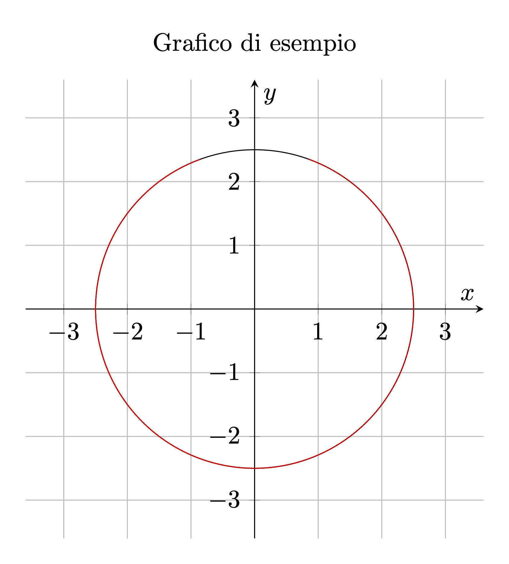
Again to appreciate the effects of Baumgarte’s stabilization we can simulate Equation 8.8 with same parameters as Example 8.1 and stabilization parameters \xi = 0.8, \omega_{\textnormal{n}} = 2. The result is showed in Figure 8.10.
Method Details
The Baumgarte method stabilizes the constraints by introducing damping into the system. Consider the following ODE:
z''(t) + 2\zeta \omega z'(t) + \omega^2 z(t) = 0,
which has the solution:
z(t) = A(t) e^{-\zeta \omega t},
where A(t) depends on the initial conditions. For 0 \leq \zeta \leq 1, the solution decays exponentially without oscillation.
Over time, numerical errors can cause the system to drift away from the constraint \Phi(x, y) of Equation 8.2 where
\Phi(x, y) = x^2+y^2-1 = 0 \tag{8.9}
To mitigate this, we use the Baumgarte stabilization method, which modifies the constraint equation to include damping terms.
The stabilized constraint equation is: \frac{\mathrm{d}^2}{\mathrm{d}t^2} \Phi(x, y) + 2\zeta \omega \frac{\mathrm{d}}{\mathrm{d}t} \Phi(x, y) + \omega^2 \Phi(x, y) = 0, where \zeta and \omega are damping parameters. For Equation 8.9 this becomes: 2x x'' + 2y y'' + 2x'^2 + 2y'^2 + 4\zeta \omega (x x' + y y') + \omega^2 (x^2 + y^2 - 1) = 0.
Modified Linear System
The stabilized system is solved using the same time-stepping approach, but with the right-hand side of the linear system modified to include the stabilization terms: r_k = 2\left[(x'_k)^2 + (y'_k)^2\right] + 4\zeta \omega (x_k x'_k + y_k y'_k) + \omega^2 (x_k^2 + y_k^2 - 1).
Inconsistent Initial Conditions: The system converges back to the constraint due to the damping terms. Initial condition x(0)=1, y(0)=v(0)=0, \color{red}u(0) = 0.1 time step \Delta t=0.01 final time t_{\max}=10. Stabilization parameters are \zeta=0.5 and \omega=1 on the left and \omega=0.1 on the right.
The pendulum example illustrates the challenges of solving DAEs numerically, particularly the issue of constraint drift. The Baumgarte stabilization method effectively mitigates this drift, ensuring long-term stability of the solution. Proper choice of damping parameters \zeta and \omega is critical for achieving optimal performance.
First-Order Pendulum DAE
Start from the motion equations
\left\{ \begin{aligned} m x^{\prime\prime}+2x\lambda=0\\ m y^{\prime\prime}+2y\lambda+mg=0\\ x^2+y^2=1 \end{aligned} \right.
divide by m and set \mu=-2\lambda/m
\left\{ \begin{aligned} x^{\prime\prime}&=\mu x\\ y^{\prime\prime}&=\mu y-g\\ x^2+y^2&=r^2\\ \end{aligned} \right.
set u=x^{\prime} and v=y^{\prime} and transform to first order
\left\{ \begin{aligned} u^{\prime} &= \mu x\\ v^{\prime} &= \mu y-g\\ x^{\prime} &= u \\ y^{\prime} &= v \\ x^2+y^2 &= r^2 \end{aligned} \right.
Derive one time the constraint
2x x^{\prime}+2y y^{\prime}=0\quad\Longrightarrow\quad xu+yv=0
Derive another time the constraint
\begin{aligned} x\dot{u}+y\dot{v}+ \dot{x}u+\dot{y}v=0\quad&\Longrightarrow\\ \mu(x^2+y^2)-gy+(u^2+v^2)=0\quad&\Longrightarrow\quad r^2\mu-gy+(u^2+v^2)=0 \end{aligned}
Derive a third time the constraint obtaining a differential equation for \mu:
\begin{aligned} r^2\dot{\mu}-gv+2(u\dot{u}+v\dot{v})&=0\quad\Longrightarrow\\ r^2\dot{\mu}-gv+2\mu(ux+vy)-2gv&=0\quad\Longrightarrow\\ r^2\dot{\mu}-3gv&=0 \end{aligned}
The DAE has index 3
NoteSummary
Original DAE
\left\{ \begin{aligned} u^{\prime}&=\mu x\\ v^{\prime}&=\mu y-g\\ x^{\prime}&=u \\ y^{\prime}&=v \\ x^2+y^2&=1 \end{aligned} \right.
hidden constraints
\begin{aligned} xu+yv & = 0\\ \mu-gy+(u^2+v^2)&=0 \end{aligned}
constraint differential equation
\mu^{\prime}-3gv=0
Unstabilized Integration
Consider the ODE without stabilization
\left\{ \begin{aligned} u^{\prime} &= \mu x\\[0.25em] v^{\prime} &= \mu y - g\\[0.25em] x^{\prime} &= u \\[0.25em] y^{\prime} &= v \\[0.25em] \mu^{\prime}&=3gv/r^2 \end{aligned} \right.
Integration with implicit Euler:
\begin{aligned} \frac{u_{k+1}-u_{k}}{h}&=\mu_{k+1}x_{k+1}\\ \frac{v_{k+1}-v_{k}}{h}&=\mu_{k+1}y_{k+1}-g \\ \frac{x_{k+1}-x_{k}}{h}&=u_{k+1} \\ \frac{y_{k+1}-y_{k}}{h}&=v_{k+1} \\ \color{blue}\frac{\mu_{k+1}-\mu_{k}}{h}&\color{blue}=\frac{3gv_{k+1}}{r^2} \end{aligned}
Solving the first four equations for x_{k+1}, y_{k+1}, u_{k+1} and v_{k+1}
\begin{aligned} c_{k+1}&= 1-h^2\mu_{k+1} \\[0.25em] x_{k+1}&=(x_k+hu_k)/c_{k+1} \\[0.25em] y_{k+1}&=(y_k+h v_k-gh^2)/c_{k+1} \\[0.25em] u_{k+1}&=(u_k+h\mu_{k+1}x_k)/c_{k+1} \\[0.25em] v_{k+1}&=(v_k+h\mu_{k+1}y_k-gh)/c_{k+1} \end{aligned}
substituting into the multiplier equation and set \delta=\mu_{k+1}-\mu_k a quadratic in \delta is obtained:
r^2h^2\delta^2 +(3gh^2y_k+r^2(h^2\mu_k-1))\delta+3gh(v_k+y_k\mu_kh-gh)=0
Choose for the solution the \delta closer to the esplicit step, i.e. \delta\approx 3hgv_k/r^2
Implicit Eulero implicito without stabilization do not work. The constraint x^2+y^2=1 is violated in few steps:
onsider the DAE without stabilization
\left\{ \begin{aligned} u^{\prime} &= \mu x\\[0.25em] v^{\prime} &= \mu y - g\\[0.25em] x^{\prime} &= u \\[0.25em] y^{\prime} &= v \\[0.25em] \color{blue} x^2+y^2&\color{blue}=r^2 \end{aligned} \right.
Using implicit Euler:
\begin{aligned} \frac{u_{k+1}-u_{k}}{h}&=\mu_{k+1}x_{k+1}\\ \frac{v_{k+1}-v_{k}}{h}&=\mu_{k+1}y_{k+1}-g \\ \frac{x_{k+1}-x_{k}}{h}&=u_{k+1} \\ \frac{y_{k+1}-y_{k}}{h}&=v_{k+1} \\ \color{blue} x_{k+1}^2+y_{k+1}^2 & \color{blue} = 1 \end{aligned}
Solving the first four equation for x_{k+1}, y_{k+1}, u_{k+1} and v_{k+1}
\begin{aligned} c_{k+1}&= 1-h^2\mu_{k+1} \\[0.25em] x_{k+1}&=(x_k+hu_k)/c_{k+1} \\[0.25em] y_{k+1}&=(y_k+h v_k-gh^2)/c_{k+1} \\[0.25em] u_{k+1}&=(u_k+h\mu_{k+1}x_k)/c_{k+1} \\[0.25em] v_{k+1}&=(v_k+h\mu_{k+1}y_k-gh)/c_{k+1} \end{aligned}
substituting into constraint a quadratic equation in \mu_{k+1} is obtained:
x_k^{2}+y_k^2-r^2 +2 h (x_k u_k+y_0 v_k) +h^2 (u_k^2+v_k^2) \\[0.5em] +g^2 h^4 -2 g h^2 (y_k+h v_k)+2h^2\mu_{k+1}-h^4\mu_{k+1}^2=0
\begin{aligned} \underbrace{[x_k^{2}+y_k^2-r^2]}_{A} +2 h \underbrace{(x_k u_k+y_0 v_k)}_{B} +h^2 (u_k^2+v_k^2) \\ +g^2 h^4 -2 g h^2 (y_k+h v_k)+2h^2\mu_{k+1}-h^4\mu_{k+1}^2=0 \end{aligned}
On the solution block (A) is zero so it is removed. Block (B) is the constraint derivative not 0 in the discretization. Thus,
2 (x_k u_k+y_0 v_k) +h (u_k^2+v_k^2) +g^2 h^3 -2 g h (y_k+h v_k)+2h\mu_{k+1}-h^3\mu_{k+1}^2=0
Solving the quadratic
\begin{aligned} \mu_{k+1}&=\frac{r\pm\sqrt{r^2+A}}{h^2r}\\[0.5em] A &= g^2h^4+2h(x_ku_k+y_kv_k)-2gh^2(y_k-hv_k)+h^2(u_k^2+v_k^2) \end{aligned}
\mu represent centripetal force maintaining mass on the constraint. Thus \mu must be negative and solving trying to avoid cancellation error:
\begin{aligned} A &= g^2h^4+2h(x_ku_k+y_kv_k)-2gh^2(y_k-hv_k)+h^2(u_k^2+v_k^2)\\[0.5em] \mu_{k+1}&=\frac{-A}{h^2(r^2+r\sqrt{r^2+A})} %%=\frac{-A}{h^2(r^2+r^2\sqrt{1+A/r^2})} =\frac{-A/r^2}{h^2(1+\sqrt{1+A/r^2})} \end{aligned}
Numerical Results
Stabilized Integration
Inplicit Euler work but it is too dissipative. Cranck-Nicolson needs stabilization. DAE transformed to ODE need a third order ODE to stabilize as follows:
\frac{\mathrm{d}^3 V(x,y)}{\mathrm{d}t^3} +a\frac{\mathrm{d}^2 V(x,y)}{\mathrm{d}t^2} +b\frac{\mathrm{d} V(x,y)}{\mathrm{d}t} +cV(x,y)=0
where V(x,y)=x^2+y^2-1. And a, b, c are chosen in such a way
z'''(t)+az''(t)+bz'(t)+cz(t)=0
satisfy \lim_{t\to\infty}z(t)=0.
Crank–Nicolson Results
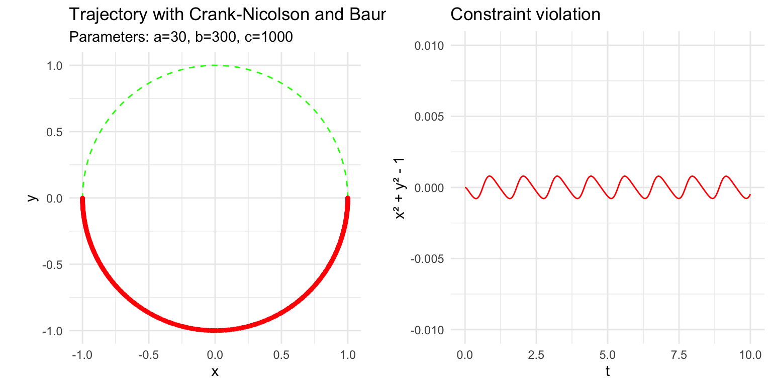
Initial consistent data and stabilizing values a=30, b=300, c=1000.
8.5 Projection Methods
Another way to stabilize the constraint
\bm{\phi}(\bm{p},t)=0
and avoid the drift effect is using the projection method. The idea is to firstly reduce the index of the DAE, thus obtaining an ODE and a list of hidden constraints. Then the resulting ODE can be numerically integrated, leading to a generic intermediate solution
\widetilde{\bm{p}}(t_n).
This temporary solution is projected to the hidden constraints in order to minimize the error between the numerical integration solution and the actual system constraints, which is a nonlinear constrained least squares problem because of the norm chosen.
It should be noticed that unlike the Baumgarte’s stabilization method this technique is useful and particularly effective if you are interested in the short term behavior, since even during transients the constraint is always satisfied. Different information from the original and reduced system can be used for various projection methods. For example, we can decide to get an advantage by first projecting the ODE solution
\widetilde{\bm{p}}(t_n)
to the position constraints and than to the velocity constraints.
Example 8.2
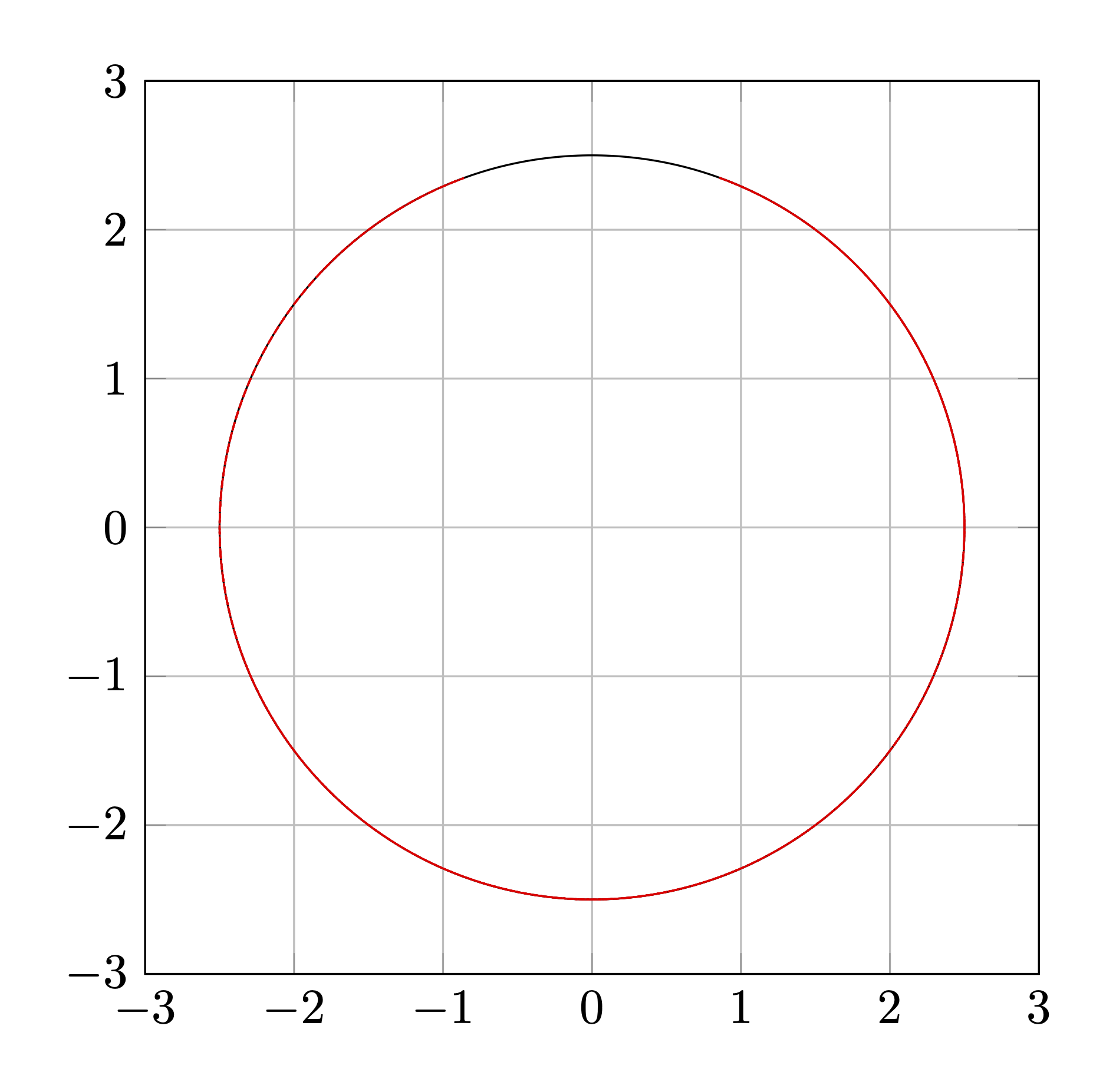
Continuing Example 8.1 we want use the Projection technique to stabilize the pendulum. The numerical scheme for integrating the reduced DAE is that in the scheme of DAEs from Lagrangian Mechanics. We want now to project the results of the generic ODE numerical integrator to the following hidden constraints,
\begin{aligned} \frac{\mathrm{d}\phi}{\mathrm{d} t} &= 2 (\bm{p}\cdot\bm{v}) = 0. \\[0.5em] \frac{\mathrm{d}^{2}\phi}{\mathrm{d} t^2} & = 2(\dot{\bm{p}}\cdot\bm{v}) + 2(\bm{p}\cdot\dot{\bm{v}}) = 2(\bm{v}\cdot\bm{v}) + 2(\bm{p}\cdot\dot{\bm{v}}) = \bm{0}. \end{aligned}
At each time step, the resulting orthogonal projection to the constraints is equal to
\begin{aligned} \text{minimize:} \quad & \frac{1}{2} \| \widetilde{\bm{p}} - \bm{p}\|^2 \\[0.5em] \text{subject to:} \quad & \bm{\phi}(\bm{p},t) = \bm{p}\cdot\bm{p} - \ell^{2} = 0 \end{aligned}
for the position coordinates projection, and
\begin{aligned} \text{minimize:} \quad & \frac{1}{2} \|\widetilde{\bm{v}} - \bm{v} \|^2 \\[0.5em] \text{subject to:} \quad & \frac{\mathrm{d}\bm{\phi}}{\mathrm{d}t}(\bm{p},t)=2(\bm{v}\cdot\bm{p})=0 \end{aligned}
for the velocity coordinates projection.
Projection Principles
Projection methods aim to leverage well-established numerical techniques to efficiently solve DAEs while ensuring consistency with their inherent constraints. The core idea is to exploit the robustness and accuracy of existing solvers for ordinary differential equations (ODEs) by transforming the problem into an ODE system with constraints and subsequently applying a projection step to maintain consistency.
Key Principles
- Utilization of existing ODE Solvers:
- Many sophisticated and highly accurate solvers are available for ODEs.
- By reformulating a DAE as an ODE, one can take advantage of these mature numerical techniques.
- Many sophisticated and highly accurate solvers are available for ODEs.
- Constraint Satisfaction via Projection:
- Directly solving a transformed ODE may lead to constraint violation over time due to numerical errors, a phenomenon known as drift.
- To mitigate drift, a projection step is introduced to enforce consistency with the hidden constraints at each step or whenever the drift becomes non-negligible.
- Directly solving a transformed ODE may lead to constraint violation over time due to numerical errors, a phenomenon known as drift.
Projection Method Workflow
The projection method follows a straightforward two-step paradigm:
- ODE Step: Advance the solution using any standard numerical solver for ODEs.
- Projection Step: Adjust the computed solution by projecting it onto the manifold defined by the constraints, thereby ensuring consistency.
This approach provides a balance between computational efficiency and constraint preservation, making it an attractive method for solving DAEs.
Requirements
The projection method relies on the following essential components:
- Index Reduction:
- DAEs often have a higher differential index, which makes them difficult to solve directly.
- Index reduction techniques are applied to convert the DAE into an ODE system with explicit algebraic constraints.
- DAEs often have a higher differential index, which makes them difficult to solve directly.
- Collection of Constraints and Jacobians:
- To perform projection, the constraints and their Jacobians must be determined.
- This involves symbolic computations to extract hidden constraints and their derivatives.
- To perform projection, the constraints and their Jacobians must be determined.
Thus, while the projection method simplifies numerical integration, it does not eliminate the need for symbolic preprocessing:
- Index reduction typically requires symbolic manipulations proportional to the index of the DAE.
- The projection step involves a smaller symbolic computation effort, primarily related to evaluating constraint Jacobians, whose complexity depends on the chosen projection algorithm.
Formulation
Consider a general DAE system:
\bm{F}(\bm{x},\bm{x}^\prime,t) = \bm{0}
where \bm{x} represents the state variables, and \bm{F} defines the differential-algebraic structure.
To facilitate numerical integration, the system is transformed into an ODE system with explicit constraints using index reduction:
\begin{aligned} \bm{x}' & = \bm{G}(\bm{x},t), \quad && \textcolor{DarkGreen}{\text{[ODE]}} \\ \bm{0} & = \bm{H}(\bm{x},t), \quad && \textcolor{DarkGreen}{\text{[Invariants or hidden constraints]}} \end{aligned}
where:
- \bm{G}(\bm{x},t) defines the transformed r.h.s. of the ODE system.
- \bm{H}(\bm{x},t) represents the constraints that must be satisfied throughout the integration process.
Projected Integration
Step 1: ODE Integration
Using an explicit numerical scheme, such as the explicit Euler method, we compute a preliminary update:
\widetilde{\bm{x}}_{k+1} = \bm{x}_{k} + \Delta t\,\bm{G}(\bm{x}_k,t_k)
where \widetilde{\bm{x}}_{k+1} is the intermediate solution, which may not satisfy the constraints due to numerical errors.
Step 2: Projection onto the Constraint Manifold
To restore consistency, the next step is to compute the corrected state \bm{x}_{k+1} by solving the constrained optimization problem:
\begin{aligned} \text{minimize} \quad & f(\textcolor{red}{\bm{z}}) = \frac{1}{2} \|\textcolor{red}{\bm{z}} - \widetilde{\bm{x}}_{k+1} \|^2 \\ \text{subject to the constraint:}\quad & \bm{H}(\textcolor{red}{\bm{z}}, t_{k+1}) = \bm{0}. \end{aligned}
then set \bm{x}_{k+1}=\textcolor{red}{\bm{z}}.
This optimization step ensures that \bm{x}_{k+1} remains on the constraint manifold, effectively eliminating the drift introduced by numerical integration.
Constrained Minimization
In many numerical applications, we encounter the problem of minimizing a function while satisfying a set of constraints. The general form of such a constrained optimization problem is:
\text{minimize} \quad f(\textcolor{red}{\bm{z}}) \quad \text{subject to} \quad \bm{h}(\textcolor{red}{\bm{z}}) = \bm{0}
where:
- f(\bm{z}) is the objective function to be minimized.
- \bm{h}(\bm{z}) represents the set of constraints that must be satisfied.
Here is shown a sketch in matlab for the solution of constrained minimization problem using function fmincon:
% Dimensione di z
n = ...;

% objective function f(z)
objective = @(z) ...;

% constraint h(z)
nonlcon = @(z) ...;

% Initial point
z0 = xtilde;

% Solve using fmincon
options = optimoptions(  'fmincon', ...
  'Display',             'iter',  ...
  'Algorithm',           'sqp',   ...
  'MaxIterations',       100,     ...
  'OptimalityTolerance', 1e-8     ...
);

z_sol = fmincon( objective, z0, ...
                 [], [], [], [], [], [], ...
                 nonlcon, options);
Solution Using Lagrange Multipliers
To find the solution, we introduce the Lagrangian function:
\mathcal{L}(\textcolor{red}{\bm{z}},\textcolor{blue}{\bm{\lambda}}) = f(\textcolor{red}{\bm{z}}) - \textcolor{blue}{\bm{\lambda}} \cdot \bm{h}(\textcolor{red}{\bm{z}})
where:
- \textcolor{blue}{\bm{\lambda}} is the vector of Lagrange multipliers, which enforces the constraints.
The necessary conditions for a solution (also called the Karush-Kuhn-Tucker conditions) correspond to the stationary points of the Lagrangian:
\left\{ \begin{aligned} \frac{\partial\mathcal{L}(\bm{z},\bm{\lambda})}{\partial\bm{z}} &= \bm{0}, \\[0.5em] \frac{\partial\mathcal{L}(\bm{z},\bm{\lambda})}{\partial\bm{\lambda}} &= \bm{0}. \end{aligned} \right.
Expanding these derivatives explicitly:
\left\{ \begin{aligned} \nabla f(\bm{z}) - \bm{h}_{\bm{z}}(\bm{z})^T \bm{\lambda} & = \bm{0}, \\[0.5em] \bm{h}(\bm{z}) & = \bm{0}. \end{aligned} \right.
where \bm{h}_{\bm{z}} is the Jacobian matrix of the constraints:
\bm{h}_{\bm{z}} = \frac{\partial \bm{h}(\bm{z})}{\partial \bm{z}}.
This system of nonlinear equations must be solved to find the optimal solution (\bm{z}, \bm{\lambda}).
Linearization of the Minimization Problem
Since the nonlinear system above is often difficult to solve directly, we employ a linearization technique around a current estimate \bm{z}. This leads to an iterative solution approach.
By performing a first-order Taylor expansion of the necessary conditions with respect to \bm{z}, we obtain:
\left\{ \begin{aligned} \nabla f(\bm{z}) + \textcolor{red}{\nabla^2 f(\bm{z}) \delta \bm{z}} - \bm{h}_{\bm{z}}(\bm{z})^T \bm{\lambda} & = \textcolor{blue}{\mathcal{O}(\|\delta \bm{z}\|^2)}, \\[0.5em] \bm{h}(\bm{z})+ \textcolor{red}{\bm{h}_{\bm{z}}(\bm{z}) \delta \bm{z}} & = \textcolor{blue}{\mathcal{O}(\|\delta \bm{\lambda}\|^2)}. \end{aligned} \right.
Ignoring the higher-order terms \mathcal{O}(\|\delta \bm{z}\|^2), we derive an iterative Newton-like method for solving the optimization problem.
Iterative Algorithm for the Constrained Minimization Problem
Initialize with an initial guess \bm{z}_0 = \widetilde{\bm{x}}_{k+1}.
Update the solution iteratively:
\bm{z}_{\ell+1} = \bm{z}_{\ell} + \delta\bm{z}, \quad \ell = 0,1,\ldots \quad \text{(until convergence)}.
Solve for the update \delta \bm{z} by solving the following linear system:
\begin{pmatrix} \nabla^2 f(\bm{z}_{\ell}) & -\bm{h}_{\bm{z}}(\bm{z}_{\ell})^T \\[0.5em] -\bm{h}_{\bm{z}}(\bm{z}_{\ell}) & \bm{0} \end{pmatrix} %%% \begin{pmatrix} \delta\bm{z}\\[0.5em] \textcolor{blue}{\bm{\lambda}} \end{pmatrix} = \begin{pmatrix} -\nabla f(\bm{z}_{\ell})\\[0.5em] \bm{h}(\bm{z}_{\ell}) \end{pmatrix}
This system provides the correction \delta\bm{z} for the next iteration step.
Special Case: Quadratic Objective Function
A particularly important case is when the objective function is quadratic, given by:
f(\bm{z}) = \frac{1}{2} \|\bm{z} - \widetilde{\bm{x}}_{k+1}\|^2.
For this choice of f(\bm{z}), the gradient and Hessian simplify to:
\nabla f(\bm{z}) = \bm{z} - \widetilde{\bm{x}}_{k+1}, \qquad \nabla^2 f(\bm{z}) = \bm{I}.
Thus, the linear system simplifies to:
\begin{pmatrix} \bm{I} & -\bm{h}_{\bm{z}}(\bm{z}_{\ell})^T \\[0.5em] -\bm{h}_{\bm{z}}(\bm{z}_{\ell}) & \bm{0} \end{pmatrix} %%% \begin{pmatrix} \delta\bm{z}\\[0.5em] \textcolor{blue}{\bm{\lambda}} \end{pmatrix} = \begin{pmatrix} \widetilde{\bm{x}}_{k+1} - \bm{z}_{\ell}\\[0.5em] \bm{h}(\bm{z}_{\ell}) \end{pmatrix}
This case is particularly useful in applications like projection methods for constrained dynamics, where \widetilde{\bm{x}}_{k+1} represents an unconstrained update that needs to be corrected to satisfy the constraints \bm{h}(\bm{z}) = \bm{0}.
A sketch in matlab for the projection solution is shown here:
n      = ...; % dimension of the problem
m      = ...; % number of constraints
xt     = ...; % point to be projected
H_fun  = @(z) ...; % The constraints m x 1 matrix
Hz_fun = @(z) ...; % Jacobian of the constraints m x n matrix
z      = xt; % initial point
for k=1:max_iter
  Hz  = Hz_fun( z );
  H   = H_fun( z );
  M   = [ eye(n), Hz.' ; Hz, zeros(n,n) ];
  b   = [ xt - z; H ];
  sol = M \ b;
  dz  = sol(1:n);
  if norm(dz,inf) < tolerance
    break;
  end
  z = z+dz;
end
8.6 Projection Algorithms
Index-1 Projection
Consider an index-1 Differential-Algebraic Equation (DAE) system of the form:
\left\{ \begin{aligned} \bm{x}' &= \bm{f}(\bm{x}, \bm{y}, t) \\[0.25em] \bm{0} &= \bm{g}(\bm{x}, \bm{y}, t) \end{aligned} \right. \tag{8.10}
where:
- \bm{x}: differential variables
- \bm{y}: algebraic variables
- \bm{f}(\bm{x}, \bm{y}, t): differential dynamics
- \bm{g}(\bm{x}, \bm{y}, t) = \bm{0}: algebraic constraints
Reformulate with Dummy Variables by introducing a dummy derivative \bm{y}_{\text{dot}}(t):
\left\{ \begin{aligned} \bm{x}'(t) &= \bm{f}(\bm{x}(t), \bm{y}(t), t) \\[0.25em] \bm{y}'(t) &= \bm{y}_{\text{dot}}(t) \\[0.25em] {\color{blue}\bm{0}} &= {\color{blue}\bm{h}(\bm{x}, \bm{y}, \bm{y}_{\text{dot}}, t)} \\[0.25em] {\color{red}\bm{0}} &= {\color{red}\bm{g}(\bm{x}, \bm{y}, t)} \end{aligned} \right.
Define:
\begin{aligned} \bm{h}(\bm{x}, \bm{y}, {\color{red}\bm{y}_{\text{dot}}}, t) &= \frac{d}{dt} \bm{g}(\bm{x}, \bm{y}, t) \\[0.5em] &= \frac{\partial \bm{g}}{\partial \bm{x}} \bm{x}' + \frac{\partial \bm{g}}{\partial \bm{y}} \bm{y}' + \frac{\partial \bm{g}}{\partial t} \\[0.5em] &= \bm{g}_{\bm{x}}(\bm{x}, \bm{y}, t)\, \bm{f}(\bm{x}, \bm{y}, t) + \bm{g}_{\bm{y}}(\bm{x}, \bm{y}, t)\, {\color{red}\bm{y}_{\text{dot}}} + \bm{g}_t(\bm{x}, \bm{y}, t) \end{aligned}
Using:
\begin{aligned} \bm{g}_{\bm{x}} &= \frac{\partial \bm{g}}{\partial \bm{x}}, \quad \bm{g}_{\bm{y}} = \frac{\partial \bm{g}}{\partial \bm{y}}, \quad \bm{g}_{t} = \frac{\partial \bm{g}}{\partial t} \end{aligned}
we solve for \bm{y}_{\text{dot}}:
{\color{red}\bm{y}_{\text{dot}}} = -\bm{g}_{\bm{y}}(\bm{x},\bm{y},t)^{-1} \left[ \bm{g}_{\bm{x}}(\bm{x},\bm{y},t)(\bm{x},\bm{y},t)\, \bm{f} + \bm{g}_t(\bm{x},\bm{y},t) \right]
Define:
\bm{e}(\bm{x}, \bm{y}, t) = -\bm{g}_{\bm{y}}(\bm{x}, \bm{y}, t)^{-1} \left[ \bm{g}_{\bm{x}}(\bm{x}, \bm{y}, t)\, \bm{f}(\bm{x}, \bm{y}, t) + \bm{g}_t(\bm{x}, \bm{y}, t) \right]
and obtain the ODE + constraint system:
\left\{ \begin{aligned} \bm{x}' &= \bm{f}(\bm{x}, \bm{y}, t) \\[0.25em] \bm{y}' &= \bm{e}(\bm{x}, \bm{y}, t) \\[0.25em] {\color{red}\bm{0}} &= {\color{red}\bm{g}(\bm{x}, \bm{y}, t)} \end{aligned} \right.
The projection method advances the ODE using any numerical integration scheme (Euler, RK, etc.) and then projects onto the constraints (red part).
Projection Phase
The system is advanced with a time integrator (e.g., Euler, Runge–Kutta), then projected onto the constraint manifold.
E.g. using Explicit Euler step:
\left\{ \begin{aligned} \widetilde{\bm{x}}_{k+1} &= \bm{x}_k + \Delta t\, \bm{f}(\bm{x}_k, \bm{y}_k, t_k) \\[0.5em] \widetilde{\bm{y}}_{k+1} &= \bm{y}_k + \Delta t\, \bm{e}(\bm{x}_k, \bm{y}_k, t_k) \end{aligned} \right.
The true solution will be
\begin{aligned} \bm{x}_{k+1} &= \widetilde{\bm{x}}_{k+1} + \delta\bm{x} \\ \bm{y}_{k+1} &= \widetilde{\bm{y}}_{k+1} + \delta\bm{y} \end{aligned}
Index-1 Projection as Minimization
Project the point (\widetilde{\bm{x}}_{k+1}, \widetilde{\bm{y}}_{k+1}) onto the constraint manifold:
\begin{aligned} \min_{\bm{x}, \bm{y}} \quad & \frac{1}{2} \left\| {\color{red}\bm{x}} - \widetilde{\bm{x}}_{k+1} \right\|^2 + \frac{1}{2} \left\| {\color{red}\bm{y}} - \widetilde{\bm{y}}_{k+1} \right\|^2 \\[1.5em] \text{subject to} \quad &\bm{g}({\color{red}\bm{x}}, {\color{red}\bm{y}}, t_{k+1}) = \bm{0} \end{aligned}
Using Lagrange multipliers, the candidate solutions are the stationary points of the Lagrangian:
\mathcal{L}(\bm{x},\bm{y},\bm{\lambda}) = \frac{1}{2}\|{\color{red}\bm{x}}-\widetilde{\bm{x}}_{k+1}\|^2+ \frac{1}{2}\|{\color{red}\bm{y}}-\widetilde{\bm{y}}_{k+1}\|^2- \bm{\lambda} \cdot \bm{g}({\color{red}\bm{x}},{\color{red}\bm{y}},t_{k+1})
which leads to the stationery conditions:
\left\{\begin{aligned} {\color{red}\bm{x}}-\widetilde{\bm{x}}_{k+1} - \bm{g}_{\bm{x}}({\color{red}\bm{x}},{\color{red}\bm{y}},t_{k+1})^T{\color{blue}\bm{\lambda}} &= \bm{0}\\[0.5em] {\color{red}\bm{y}}-\widetilde{\bm{y}}_{k+1} - \bm{g}_{\bm{y}}({\color{red}\bm{x}},{\color{red}\bm{y}},t_{k+1})^T{\color{blue}\bm{\lambda}} &= \bm{0}\\[0.5em] \bm{g}({\color{red}\bm{x}},{\color{red}\bm{y}},t_{k+1}) &= \bm{0} \end{aligned}\right.
Newton’s Method for Projection
Use Newton (like) iterations to solve the nonlinear system. Set
\bm{x}_{k+1} = \widetilde{\bm{x}}_{k+1}+ \delta\bm{x} \quad\text{and}\quad \bm{y}_{k+1} = \widetilde{\bm{y}}_{k+1}+ \delta\bm{y}
after linearization neglecting high order term the Newton like iterative method become:
Initialization \ell\leftarrow 0
\begin{aligned} \bm{x}^{(\ell)} & = \widetilde{\bm{x}}_{k+1} \\ \bm{y}^{(\ell)} & = \widetilde{\bm{y}}_{k+1} \end{aligned}
Solve:
\begin{aligned} \begin{pmatrix} \bm{I} & \bm{0} & -\bm{g}_{\bm{x}}^T \\[0.25em] \bm{0} & \bm{I} & -\bm{g}_{\bm{y}}^T \\[0.25em] -\bm{g}_{\bm{x}} & -\bm{g}_{\bm{y}} & \bm{0} \end{pmatrix} \begin{pmatrix} \delta\bm{x} \\[0.25em] \delta\bm{y} \\[0.25em] \bm{\lambda} \end{pmatrix} = \begin{pmatrix} \widetilde{\bm{x}}_{k+1} - \bm{x}^{(\ell)} \\[0.5em] \widetilde{\bm{y}}_{k+1} - \bm{y}^{(\ell)} \\[0.5em] \bm{g}(\bm{x}^{(\ell)}, \bm{y}^{(\ell)}, t_ {k+1}) \end{pmatrix} \end{aligned}
Update:
\begin{aligned} \bm{x}^{(\ell+1)} &= \bm{x}^{(\ell)} + \delta\bm{x}, \\ \bm{y}^{(\ell+1)} &= \bm{y}^{(\ell)} + \delta\bm{y} \end{aligned}
\ell\leftarrow\ell+1 and repeat step 2 and 3 until convergence.
Index-2 Projection
An index-2 differential-algebraic equation (DAE) can be written as:
\left\{\begin{aligned} \bm{x}'& = \bm{f}(\bm{x},\bm{y},t) \\[0.5em] \bm{0} & = \bm{g}(\bm{x},t) \end{aligned}\right.
where:
- \bm{x} and \bm{y} are the differential and algebraic variables;
- \bm{f}(\bm{x}, \bm{y}, t) is the right-hand side of the differential equations;
- \bm{g}(\bm{x}, t) encodes the algebraic constraints.
Constraint Differentiation
To regularize the system, differentiate the constraint and introduce a dummy derivative for \bm{y}:
\left\{\begin{aligned} \bm{x}'(t)& = \bm{f}(\bm{x}(t),\bm{y}(t),t) \\[0.5em] \bm{y}'(t) & = \bm{y}_{\text{dot}}(t) \\[0.5em] \color{DarkGreen}\bm{0} & = \color{DarkGreen}\bm{a}(\bm{x},\bm{y},t) + \bm{g}_{\bm{x}}(\bm{x},t)\bm{f}_{\bm{y}}(\bm{x},\bm{y},t)\bm{y}_{\text{dot}} \\[0.5em] \color{blue}\bm{0} & = \color{blue}\bm{h}(\bm{x},\bm{y},t) \\[0.5em] \color{red}\bm{0} & = \color{red}\bm{g}(\bm{x},t) \end{aligned}\right.
where
First hidden constraint \begin{aligned} \bm{0}&= \frac{\mathrm{d}}{\mathrm{d}t}\bm{g}(\bm{x},t) \\[0.5em] & = \bm{g}_{\bm{x}}(\bm{x},t)\bm{f}(\bm{x},\bm{y},t)+ \bm{g}_t(\bm{x},t) \\[0.5em] &= \bm{h}(\bm{x},\bm{y},t) \end{aligned}
Second hidden constraint \begin{aligned} \bm{0} &=\frac{\mathrm{d}}{\mathrm{d}t}\bm{h}(\bm{x},\bm{y},t)\\[0.5em] & = \underbrace{\bm{h}_{\bm{x}}(\bm{x},\bm{y},t)\bm{f}(\bm{x},\bm{y},t)+ \bm{h}_t(\bm{x},\bm{y},t)}_{ \bm{a}(\bm{x},\bm{y},t) }+ \underbrace{\bm{h}_{\bm{y}}(\bm{x},\bm{y},t)}_{ \bm{g}_{\bm{x}}(\bm{x},t)\bm{f}_{\bm{y}}(\bm{x},\bm{y},t) } \bm{y}_{\text{dot}} \end{aligned}
Solving for \bm{y}_{\text{dot}} gives the regularized system:
\left\{\begin{aligned} \bm{x}'(t) & = \bm{f}(\bm{x},\bm{y},t) \\[0.5em] \bm{y}'(t) & = -\Big[\bm{g}_{\bm{x}}(\bm{x},t)\bm{f}_{\bm{y}}(\bm{x},\bm{y},t)\Big]^{-1} \bm{a}_{\bm{x}}(\bm{x},\bm{y},t) \\[0.5em] \color{blue}\bm{0} & = \color{blue}\bm{h}(\bm{x},\bm{y},t) \\[0.5em] \color{red}\bm{0} & = \color{red}\bm{g}(\bm{x},t) \end{aligned}\right.
an ODE with hidden constraints.
Numerical Solution
The system is solved using a numerical method (e.g., Euler or Runge-Kutta) followed by a projection step to enforce the constraints.
Explicit Euler Step Example
Advance solution
\left\{\begin{aligned} \bm{x}_{k+1} & = \bm{x}_{k}+\Delta t\,\bm{f}(\bm{x}_k,\bm{y}_k,t_k) \\[0.5em] \bm{y}_{k+1} & = \bm{y}_{k}-\Delta t\, \Big[\bm{g}_{\bm{x}}(\bm{x}_k,t_k)\bm{f}_{\bm{y}}(\bm{x}_k,\bm{y}_k,t_k)\Big]^{-1} \bm{a}_{\bm{x}}(\bm{x}_k,\bm{y}_k,t_k) \end{aligned}\right.
Project onto Constraints:
Solve the constrained minimization problem:\begin{aligned} \text{minimize}\qquad & \frac{1}{2} \left\| {\color{red}\bm{x}}-\widetilde{\bm{x}}_{k+1} \right\|^2 + \frac{1}{2} \left\| {\color{red}\bm{y}}-\widetilde{\bm{y}}_{k+1} \right\|^2 \\[2em] \text{subject to}\qquad & \left\{\begin{array}{l} \bm{g}({\color{red}\bm{x}},t_{k+1}) = \bm{0}\\[0.5em] \bm{h}({\color{red}\bm{x}},{\color{red}\bm{y}},t_{k+1}) = \bm{0} \end{array}\right. \end{aligned}
This is solved using Lagrange multipliers and linearization.
Projection algorithm
Using Lagrange multiplier:
\begin{aligned} \mathcal{L}({\color{red}\bm{x}},{\color{red}\bm{y}},{\color{blue}\bm{\lambda}},{\color{blue}\bm{\mu}}) & = \frac{1}{2}\|{\color{red}\bm{x}}-\widetilde{\bm{x}}_{k+1}\|^2+ \frac{1}{2}\|{\color{red}\bm{y}}-\widetilde{\bm{y}}_{k+1}\|^2 \\[0.5em] & -{\color{blue}\bm{\lambda}}\cdot\bm{g}({\color{red}\bm{x}},t_{k+1}) -{\color{blue}\bm{\mu}}\cdot\bm{h}({\color{red}\bm{x}},{\color{red}\bm{y}},t_{k+1}) \end{aligned}
or the solution of the non linear system:
\frac{\partial\mathcal{L}}{\partial\bm{x}} = \bm{0},\quad \frac{\partial\mathcal{L}}{\partial\bm{y}} = \bm{0},\quad \frac{\partial\mathcal{L}}{\partial\bm{\lambda}} =\bm{0},\quad \frac{\partial\mathcal{L}}{\partial\bm{\mu}} = \bm{0}.
that written explicitly is \left\{\begin{aligned} {\color{red}\bm{x}}-\widetilde{\bm{x}}_{k+1} - \bm{g}_{\bm{x}}({\color{red}\bm{x}},t_{k+1})^T{\color{blue}\bm{\lambda}} - \bm{h}_{\bm{x}}({\color{red}\bm{x}},{\color{red}\bm{y}},t_{k+1})^T{\color{blue}\bm{\mu}} &= \bm{0} \\[0.5em] {\color{red}\bm{y}}-\widetilde{\bm{y}}_{k+1} - \bm{h}_{\bm{y}}({\color{red}\bm{x}},{\color{red}\bm{y}},t_{k+1})^T{\color{blue}\bm{\mu}} &= \bm{0} \\[0.5em] \bm{g}({\color{red}\bm{x}},t_{k+1}) &= \bm{0} \\[0.5em] \bm{h}({\color{red}\bm{x}},{\color{red}\bm{y}},t_{k+1}) &= \bm{0} \end{aligned}\right.
after linearization do until convergence (\ell = 0,1,\ldots) the following iterations
Initialization \ell\leftarrow 0 \begin{aligned} \bm{x}^{(\ell)} & = \widetilde{\bm{x}}_{k+1},\\ \bm{y}^{(\ell)} & = \widetilde{\bm{y}}_{k+1} \end{aligned}
Solve \begin{pmatrix} \bm{I} & \bm{0} & -\bm{g}_{\bm{x}}^T & -\bm{h}_{\bm{x}}^T \\[0.5em] \bm{0} & \bm{I} & \bm{0} & -\bm{h}_{\bm{y}}^T \\[0.5em] -\bm{g}_{\bm{x}} & \bm{0} & \bm{0} & \bm{0}\\[0.5em] -\bm{h}_{\bm{x}} & -\bm{h}_{\bm{y}} & \bm{0} & \bm{0} \end{pmatrix} %%% \begin{pmatrix} \delta\bm{x}\\[0.5em] \delta\bm{y}\\[0.5em] \color{blue}\bm{\lambda} \\[0.5em] \color{blue}\bm{\mu} \end{pmatrix} = \begin{pmatrix} \widetilde{\bm{x}}_{k+1}-\bm{x}^{(\ell)}\\[0.5em] \widetilde{\bm{y}}_{k+1}-\bm{y}^{(\ell)}\\[0.5em] \bm{g}(\bm{x}^{(\ell)},t_{k+1})\\[0.5em] \bm{h}(\bm{x}^{(\ell)},\bm{y}^{(\ell)},t_{k+1}) \end{pmatrix}
Advance:
\begin{aligned} \bm{x}^{(\ell+1)} & = \bm{x}^{(\ell)} + \delta\bm{x}, \\ \bm{y}^{(\ell+1)} & = \bm{y}^{(\ell)} + \delta\bm{y}, \end{aligned}
\ell\leftarrow\ell+1 and repeat step 2 and 3 until convergence.
Approximate Projection algorithm
To speed up computation we can project separately position and velocity solving two consecutive project:
x projection:
\begin{aligned} \text{minimize}\qquad & \frac{1}{2} \left\| {\color{red}\bm{x}}-\widetilde{\bm{x}}_{k+1} \right\|^2 \\[0.5em] \text{subject to}\qquad & \bm{g}({\color{red}\bm{x}},t_{k+1}) = \bm{0} \end{aligned}
y projection:
\begin{aligned} \text{minimize}\qquad & \frac{1}{2} \left\| {\color{red}\bm{y}}-\widetilde{\bm{y}}_{k+1} \right\|^2 \\[0.5em] \text{subject to}\qquad & \bm{h}(\bm{x}_{k+1},{\color{red}\bm{y}},t_{k+1}) = \bm{0} \end{aligned}
Using Lagrange multiplier we obtain the two nonlinear system to be solved
x problem: \left\{\begin{aligned} {\color{red}\bm{x}}-\widetilde{\bm{x}}_{k+1} - \bm{g}_{\bm{x}}({\color{red}\bm{x}},t_{k+1})^T{\color{blue}\bm{\lambda}} &= \bm{0} \\[0.5em] \bm{g}({\color{red}\bm{x}},t_{k+1}) &= \bm{0} \end{aligned}\right.
Initialization \ell\leftarrow 0
\bm{x}^{(\ell)} = \widetilde{\bm{x}}_{k+1}
Solve \begin{pmatrix} \bm{I} & -\bm{g}_{\bm{x}}^T \\[0.5em] -\bm{g}_{\bm{x}} & \bm{0} \end{pmatrix} %%% \begin{pmatrix} \delta\bm{x}\\[0.5em] \color{blue}\bm{\lambda} \end{pmatrix} = \begin{pmatrix} \widetilde{\bm{x}}_{k+1}-\bm{x}^{(\ell)}\\[0.5em] \bm{g}(\bm{x}^{(\ell)},t_{k+1}) \end{pmatrix}
Advance:
\bm{x}^{(\ell+1)} = \bm{x}^{(\ell)} + \delta\bm{x}
- \ell\leftarrow\ell+1 and repeat step 2 and 3 until convergence.
y problem: \left\{\begin{aligned} {\color{red}\bm{y}}-\widetilde{\bm{y}}_{k+1} - \bm{h}_{\bm{y}}({\color{red}\bm{x}},{\color{red}\bm{y}},t_{k+1})^T{\color{blue}\bm{\mu}} &= \bm{0} \\[0.5em] \bm{h}({\color{red}\bm{x}},{\color{red}\bm{y}},t_{k+1}) &= \bm{0} \end{aligned}\right.
Initialization \ell\leftarrow 0 \bm{y}^{(\ell)} = \widetilde{\bm{y}}_{k+1}
Solve \begin{pmatrix} \bm{I} & -\bm{h}_{\bm{y}}^T \\[0.5em] -\bm{h}_{\bm{y}} & \bm{0} \end{pmatrix} %%% \begin{pmatrix} \delta\bm{y}\\[0.5em] \color{blue}\bm{\mu} \end{pmatrix} = \begin{pmatrix} \widetilde{\bm{y}}_{k+1}-\bm{y}^{(\ell)}\\[0.5em] \bm{h}(\bm{x}^{(\ell)},\bm{y}^{(\ell)},t_{k+1}) \end{pmatrix}
Advance:
\bm{y}^{(\ell+1)} = \bm{y}^{(\ell)} + \delta\bm{y},
\ell\leftarrow\ell+1 and repeat step 2 and 3 until convergence.
Index-3 Projection
An Index-3 DAE typically arises in mechanical systems with constraints, such as: \left\{\begin{aligned} \bm{p}'& = \bm{v} \\[0.25em] \bm{M}(\bm{p},\bm{v},t)\bm{v}'+\bm{\Phi}_{\bm{p}}(\bm{p},t)^T\bm{\lambda} & = \bm{f}(\bm{p},\bm{v},t) \\[0.25em] \bm{\Phi}(\bm{p},t) & = \bm{0} \end{aligned}\right.
where:
\bm{p} and \bm{v} are the position and velocity variables,
\bm{M} is the mass matrix,
\bm{\Phi} represents the constraints,
\bm{\lambda} are the Lagrange multipliers.
To handle the higher-index constraints, we introduce dummy variables and differentiate the constraints
\left\{\begin{aligned} \bm{p}'(t) &= \bm{v}(t), \\[0.25em] \bm{v}'(t) &= \bm{v}_{\text{dot}} \\[0.5em] & \text{Index one part (solve for $\bm{v}_{\text{dot}}$ and $\bm{\lambda}$)} \\ \bm{0} &= \bm{M}(\bm{p},\bm{v},t)\bm{v}_{\text{dot}}+\bm{\Phi}_{\bm{p}}(\bm{p},t)^T\bm{\lambda} - \bm{f}(\bm{p},\bm{v},t) \\[0.25em] \color{DarkGreen}\bm{0}&= \color{DarkGreen}\bm{\Phi}_{\bm{p}}(\bm{p},t)\bm{v}_{\text{dot}}+ \bm{a}(\bm{p},\bm{v},t) \\[0.5em] & \text{Hidden constraints (projection for $\bm{p}$ and $\bm{v}$)} \\ \color{blue}\bm{0} &= \color{blue}\bm{h}(\bm{p},\bm{v},t), \\ \color{red}\bm{0} &= \color{red}\bm{\Phi}(\bm{p},t) \end{aligned}\right.
where
\begin{aligned} \bm{h}(\bm{p},\bm{v},t) & = \frac{\mathrm{d}}{\mathrm{d}t}\bm{\Phi}(\bm{p},t) \\ & = \bm{\Phi}_{\bm{p}}(\bm{x},t)\bm{v}+\bm{\Phi}_t(\bm{p},t) \\[0.5em] \bm{a}(\bm{p},\bm{v},t) & = \bm{h}_{\bm{p}}(\bm{p},\bm{v},t)\bm{v}+ \bm{h}_t(\bm{p},\bm{v},t) \end{aligned}
By solving for \bm{v}_{\text{dot}} and \bm{\lambda} we obtain the reduced ODE system:
\left\{\begin{aligned} \bm{p}' & = \bm{v} \\[0.5em] \bm{v}' & = \bm{v}_{\text{dot}}(\bm{p},\bm{v},t) \end{aligned}\right.
where \bm{v}_{\text{dot}} is obtained from \bm{p} and \bm{v} by solving the linear system:
\begin{pmatrix} \bm{M}(\bm{p},\bm{v},t) & \bm{\Phi}_{\bm{p}}(\bm{p},t)^T \\[0.5em] \bm{\Phi}_{\bm{p}}(\bm{p},t) & \bm{0} \end{pmatrix} \begin{pmatrix} \bm{v}_{\text{dot}} \\[0.5em] \bm{\lambda} \end{pmatrix} = \begin{pmatrix} \bm{f}(\bm{p},\bm{v},t) \\[0.5em] -\bm{a}(\bm{p},\bm{v},t) \end{pmatrix}
The invariants
\left\{\begin{aligned} \color{blue}\bm{0} & = \color{blue}\bm{h}(\bm{p},\bm{v},t) \\[0.5em] \color{red}\bm{0} & = \color{red}\bm{\Phi}(\bm{p},t) \end{aligned}\right.
are used in the projection step.
Index-3 Advancement
Projection method advance the ODE using any numerical method (Euler, RK, …) and next project onto the constraints (red and blue part).
E.g. using Explicit Euler step:
\left\{\begin{aligned} \bm{p}_{k+1} & = \bm{p}_{k} + \Delta t \,\bm{v}_k \\[0.5em] \bm{v}_{k+1} & = \bm{v}_{k} + \Delta t \,(\bm{v}_{\text{dot}})_k \end{aligned}\right.
where \bm{v}_{\text{dot}} is obtained from \bm{p}_k and \bm{v}_k by solving the linear system:
\begin{pmatrix} \bm{M}(\bm{p}_k,\bm{v}_k,t_k) & \bm{\Phi}_{\bm{p}}(\bm{p}_k,t_k)^T \\[0.5em] \bm{\Phi}_{\bm{p}}(\bm{p}_k,t_k) & \bm{0} \end{pmatrix} \begin{pmatrix} \bm{v}_{\text{dot}} \\[0.5em] \bm{\lambda} \end{pmatrix} = \begin{pmatrix} \bm{f}(\bm{p}_k,\bm{v}_k,t_k) \\[0.5em] -\bm{a}(\bm{p}_k,\bm{v}_k,t_k) \end{pmatrix}
Index-3 Projection
The projection phase solve the problem \begin{aligned} \text{minimize}\qquad & \frac{1}{2} \left\| {\color{red}\bm{p}}-\widetilde{\bm{p}}_{k+1} \right\|^2 + \frac{1}{2} \left\| {\color{red}\bm{v}}-\widetilde{\bm{v}}_{k+1} \right\|^2 \\[0.5em] \text{subject to}\qquad & \left\{ \begin{aligned} \bm{\Phi}({\color{red}\bm{p}},t_{k+1}) = \bm{0}\\[0.25em] \bm{h}({\color{red}\bm{p}},{\color{red}\bm{v}},t_{k+1}) = \bm{0} \end{aligned} \right. \end{aligned}
using Lagrange multiplier:
\begin{aligned} \mathcal{L}({\color{red}\bm{p}},{\color{red}\bm{v}},{\color{blue}\bm{\lambda}},{\color{blue}\bm{\mu}}) &= \frac{1}{2}\|{\color{red}\bm{p}}-\widetilde{\bm{p}}_{k+1}\|^2+ \frac{1}{2}\|{\color{red}\bm{v}}-\widetilde{\bm{v}}_{k+1}\|^2 \\[0.5em] & -{\color{blue}\bm{\lambda}}\cdot\bm{\Phi}({\color{red}\bm{x}},t_{k+1}) -{\color{blue}\bm{\mu}}\cdot\bm{h}({\color{red}\bm{x}},{\color{red}\bm{y}},t_{k+1}) \end{aligned}
or the solution of the non linear system:
\frac{\partial\mathcal{L}}{\partial\bm{p}} = \frac{\partial\mathcal{L}}{\partial\bm{v}} = \frac{\partial\mathcal{L}}{\partial\bm{\lambda}} = \frac{\partial\mathcal{L}}{\partial\bm{\mu}} = \bm{0}.
Use Newton (like) iterations to solve the nonlinear system. Set
\bm{p}_{k+1} = \widetilde{\bm{p}}_{k+1}+ \delta\bm{p} \quad\text{and}\quad \bm{v}_{k+1} = \widetilde{\bm{v}}_{k+1}+ \delta\bm{v}
after linearization neglecting high order term the Newton like iterative method become:
Initialization \ell\leftarrow 1
\bm{p}^{(\ell)} = \widetilde{\bm{p}}_{k+1} \quad \text{and} \quad \bm{v}^{(\ell)} = \widetilde{\bm{v}}_{k+1}
Solve:
\begin{pmatrix} \bm{I} & \bm{0} & -\bm{\Phi}_{\bm{p}}^T & -\bm{h}_{\bm{p}}^T \\[0.25em] \bm{0} & \bm{I} & \bm{0} & -\bm{h}_{\bm{v}}^T \\[0.35em] -\bm{\Phi}_{\bm{p}} & \bm{0} & \bm{0} & \bm{0}\\[0.25em] -\bm{h}_{\bm{p}} & -\bm{h}_{\bm{v}} & \bm{0} & \bm{0} \end{pmatrix} %%% \begin{pmatrix} \delta\bm{p}\\[0.25em] \delta\bm{v}\\[0.25em] \color{blue}\bm{\lambda} \\[0.25em] \color{blue}\bm{\mu} \end{pmatrix} = \begin{pmatrix} \widetilde{\bm{p}}_{k+1}-\bm{p}^{(\ell)}\\[0.25em] \widetilde{\bm{v}}_{k+1}-\bm{v}^{(\ell)}\\[0.25em] \bm{\Phi}(\bm{p}^{(\ell)},t_{k+1})\\[0.25em] \bm{h}(\bm{p}^{(\ell)},\bm{v}^{(\ell)},t_{k+1}) \end{pmatrix}
Update:
\begin{aligned} \bm{p}^{(\ell+1)} &= \bm{p}^{(\ell)} + \delta\bm{p}, \\ \bm{v}^{(\ell+1)} &= \bm{v}^{(\ell)} + \delta\bm{v} \end{aligned}
Repeat step 2 and 3 until convergence.
Approximate Projection
Position Projection
\begin{aligned} \text{minimize}\qquad & \frac{1}{2} \left|\left|{\color{red}\bm{p}}-\widetilde{\bm{p}}_{k+1}\right|\right|^2 \\ \text{subject to}\qquad & \bm{\Phi}({\color{red}\bm{p}},t_{k+1}) = \bm{0} \end{aligned}
using Lagrange multiplier:
\mathcal{L}({\color{red}\bm{p}},{\color{blue}\bm{\lambda}}) = \frac{1}{2}||{\color{red}\bm{p}}-\widetilde{\bm{p}}_{k+1}||^2 -{\color{blue}\bm{\lambda}}\cdot\bm{\Phi}({\color{red}\bm{p}},t_{k+1})
or find the solution of the non linear system:
\frac{\partial\mathcal{L}}{\partial\bm{p}} = \bm{0},\quad \frac{\partial\mathcal{L}}{\partial\bm{\lambda}} = \bm{0}.
Velocity Projection
\begin{aligned} \text{minimize}\qquad & \frac{1}{2} \left\|{\color{red}\bm{v}}-\widetilde{\bm{v}}_{k+1}\right\|^2 \\ \text{subject to}\qquad & \bm{h}(\bm{p}_{k+1},{\color{red}\bm{v}},t_{k+1}) = \bm{0} \end{aligned}
using Lagrange multiplier:
\mathcal{L}({\color{red}\bm{v}},{\color{blue}\bm{\mu}}) = \frac{1}{2}|{\color{red}\bm{v}}-\widetilde{\bm{v}}_{k+1}||^2 -{\color{blue}\bm{\mu}}\cdot\bm{h}(\bm{p}_{k+1},{\color{red}\bm{v}},t_{k+1})
or the solution of the non linear system:
\frac{\partial\mathcal{L}}{\partial\bm{v}} = \bm{0},\qquad \frac{\partial\mathcal{L}}{\partial\bm{\mu}} = \bm{0}.
\bm{p}^{(0)} = \widetilde{\bm{p}}_{k+1},\qquad \bm{p}^{(\ell+1)} = \bm{p}^{(\ell)} + \delta\bm{p},
\bm{v}^{(0)} = \widetilde{\bm{v}}_{k+1},\qquad \bm{v}^{(\ell+1)} = \bm{v}^{(\ell)} + \delta\bm{v},
\begin{pmatrix} \bm{I} & -\bm{\Phi}_{\bm{p}}^T \\[0.5em] -\bm{\Phi}_{\bm{p}} & \bm{0} \end{pmatrix} %%% \begin{pmatrix} \delta\bm{p}\\[0.5em] \color{blue}\bm{\lambda} \end{pmatrix} = \begin{pmatrix} \widetilde{\bm{p}}_{k+1}-\bm{p}^{(\ell)}\\[0.5em] \bm{\Phi}(\bm{p}^{(\ell)},t_{k+1}) \end{pmatrix}
\begin{pmatrix} \bm{I} & -\bm{h}_{\bm{v}}^T \\[0.5em] -\bm{h}_{\bm{v}} & \bm{0} \end{pmatrix} %%% \begin{pmatrix} \delta\bm{v}\\[0.5em] \color{blue}\bm{\mu} \end{pmatrix} = \begin{pmatrix} \widetilde{\bm{v}}_{k+1}-\bm{v}^{(\ell)}\\[0.5em] \bm{h}(\bm{p}_{k+1},\bm{v}^{(\ell)},t_{k+1}) \end{pmatrix}
where \bm{h}_{\bm{v}}=\bm{h}_{\bm{v}}(\bm{p}_{k+1},\bm{v}^{(\ell)},t_{k+1}) and \bm{\Phi}_{\bm{p}}=\bm{\Phi}(\bm{p}^{(\ell)},t_{k+1}).
8.7 Implicit Projection
Index-1 DAE
Consider a semi-explicit DAE (with index > 1):
\left\{\begin{aligned} \bm{z}' &= \bm{f}(\bm{z}, \bm{w}, t) \\[0.5em] \bm{0} &= \bm{g}(\bm{z}, \bm{w}, t) \end{aligned}\right.
This system can be transformed into an index-1 DAE by index reduction, along with invariants:
\text{Index-1 DAE:}\left\{\begin{aligned} \bm{x}' &= \bm{f}(\bm{x}, \bm{y}, t) \\[0.5em] \bm{0} &= \bm{a}(\bm{x}, \bm{y}, t) \end{aligned}\right. \qquad \underbrace{\bm{b}(\bm{x}, \bm{y}, t) = \bm{0}}_{\text{invariants}}
The index-1 system is then solved as an implicitly defined ODE:
\bm{x}' = \bm{F}(\bm{x}, t)
where \bm{F}(\bm{x}, t) = \bm{f}(\bm{x}, \bm{y}(\bm{x}, t), t) and \bm{y}(\bm{x}, t) is the solution to the equation \bm{b}(\bm{x}, \bm{y}, t) = \bm{0}.
Explicit Advancement
Explicit methods, such as the explicit Euler method, do not require complex handling. The update step is given by:
\bm{x}_{k+1} = \bm{x}_k + \Delta t \bm{F}(\bm{x}_k, t_k)
The evaluation of \bm{F}(\bm{x}_k, t_k) proceeds as follows:
Solve \bm{h}({\color{red}\bm{y}}) = \bm{a}(\bm{x}_k, {\color{red}\bm{y}}, t_k) = \bm{0} to compute \bm{y}_k.
Compute \bm{F}(\bm{x}_k, t_k) = \bm{f}(\bm{x}_k, \bm{y}_k, t_k).
Implicit Advancement
For implicit methods, such as implicit Euler, the update step is:
\bm{x}_{k+1} = \bm{x}_k + \Delta t \bm{F}(\bm{x}_{k+1}, t_{k+1})
This requires solving the implicit equation:
\bm{G}({\color{red}\bm{z}}) = {\color{red}\bm{z}} - \Delta t \bm{F}({\color{red}\bm{z}}, t_{k+1}) - \bm{x}_k = \bm{0}
The solution of \bm{G}({\color{red}\bm{z}}) = 0 requires an iterative method such as Newton-Raphson:
{\color{red}\bm{z}}^{(\ell+1)} = {\color{red}\bm{z}}^{(\ell)} - \left(\frac{\partial \bm{G}({\color{red}\bm{z}}^{(\ell)})}{\partial {\color{red}\bm{z}}}\right)^{-1} \bm{G}({\color{red}\bm{z}}^{(\ell)})
This method requires the Jacobian of \bm{F}(\bm{x}, t):
\frac{\partial \bm{G}({\color{red}\bm{z}})}{\partial {\color{red}\bm{z}}} = \bm{I} - \Delta t \frac{\partial \bm{F}({\color{red}\bm{z}}, t_{k+1})}{\partial {\color{red}\bm{z}}}
RHS Jacobian
Given the system
\bm{F}(\bm{x}, t) = \bm{f}(\bm{x}, \bm{y}(\bm{x}, t), t), \qquad \bm{a}(\bm{x}, \bm{y}(\bm{x}, t), t) = \bm{0},
we can derive the following expressions for the Jacobian:
\left\{ \begin{aligned} \frac{\partial \bm{F}(\bm{x}, t)}{\partial \bm{x}} &= \frac{\partial \bm{f}(\bm{x}, \bm{y}, t)}{\partial \bm{x}} + \frac{\partial \bm{f}(\bm{x}, \bm{y}, t)}{\partial \bm{y}} \frac{\partial \bm{y}(\bm{x}, t)}{\partial \bm{x}} \\[0.5em] \bm{0} &= \frac{\partial \bm{a}(\bm{x}, \bm{y}, t)}{\partial \bm{x}} + \frac{\partial \bm{a}(\bm{x}, \bm{y}, t)}{\partial \bm{y}} \frac{\partial \bm{y}(\bm{x}, t)}{\partial \bm{x}} \end{aligned} \right.
From this, we can express the derivative of \bm{y}(\bm{x}, t) with respect to \bm{x} as:
\frac{\partial \bm{y}(\bm{x}, t)}{\partial \bm{x}} = -\bm{a}_{\bm{y}}(\bm{x}, \bm{y}, t)^{-1} \bm{a}_{\bm{x}}(\bm{x}, \bm{y}, t),
and the Jacobian of \bm{F}(\bm{x}, t) becomes:
\boxed{ \frac{\partial \bm{F}(\bm{x}, t)}{\partial \bm{x}} = \bm{f}_{\bm{x}}(\bm{x}, \bm{y}, t) - \bm{f}_{\bm{y}}(\bm{x}, \bm{y}, t) \bm{a}_{\bm{y}}(\bm{x}, \bm{y}, t)^{-1} \bm{a}_{\bm{x}}(\bm{x}, \bm{y}, t) }
Jacobian Computation
In practice, the Jacobian should be computed as follows:
Start with the system:
\bm{F}(\bm{x}, t) = \bm{f}(\bm{x}, \bm{y}(\bm{x}, t), t), \qquad \bm{a}(\bm{x}, \bm{y}(\bm{x}, t), t) = \bm{0}.
Solve for \bm{Z} by solving the linear system:
\bm{a}_{\bm{y}}(\bm{x}, \bm{y}, t) \bm{Z} = - \bm{a}_{\bm{x}}(\bm{x}, \bm{y}, t)
Compute the Jacobian:
\frac{\partial \bm{F}(\bm{x}, t)}{\partial \bm{x}} = \bm{f}_{\bm{x}}(\bm{x}, \bm{y}, t) + \bm{f}_{\bm{y}}(\bm{x}, \bm{y}, t) \bm{Z}
Index-3 DAEs
We begin with the following system of differential-algebraic equations (DAEs):
\left\{ \begin{aligned} \bm{p}' &= \bm{v} \\[0.5em] \bm{M}(\bm{p}, \bm{v}, t) \bm{v}' + \bm{\Phi}_{\bm{p}}(\bm{p}, t)^T \bm{\lambda} &= \bm{f}(\bm{p}, \bm{v}, t) \\[0.5em] \bm{\Phi}(\bm{p}, t) &= \bm{0} \end{aligned} \right.
Defining Functions for RHS and Invariants
Let us introduce the following functions to represent the system:
- Function F:
\bm{F}(\bm{p}, \bm{v}, {\color{red}\bm{v}_{\mathrm{dot}}}, {\color{red}\bm{\lambda}}, t) = \bm{M}(\bm{p}, \bm{v}, t) {\color{red}\bm{v}_{\mathrm{dot}}} + \bm{\Phi}_{\bm{p}}(\bm{p}, t)^T {\color{red}\bm{\lambda}} - \bm{f}(\bm{p}, \bm{v}, t)
- Function G:
\bm{G}(\bm{p}, \bm{v}, {\color{red}\bm{v}_{\mathrm{dot}}}, t) = \bm{\Phi}_{\bm{p}}(\bm{p}, t) {\color{red}\bm{v}_{\mathrm{dot}}} + \bm{a}(\bm{p}, \bm{v}, t)
Thus, the system can be expressed as:
\begin{aligned} \bm{F}(\bm{p}, \bm{v}, {\color{red}\bm{v}_{\mathrm{dot}}(\bm{p}, \bm{v}, t)}, {\color{red}\bm{\lambda}(\bm{p}, \bm{v}, t)}, t) &= \bm{0} \\[0.5em] \bm{G}(\bm{p}, \bm{v}, {\color{red}\bm{v}_{\mathrm{dot}}(\bm{p}, \bm{v}, t)}, t) &= \bm{0} \end{aligned}
Jacobian Derivatives of Functions F and G
Taking derivatives of \bm{F} and \bm{G} with respect to \bm{p}, we obtain the following system of equations:
\begin{aligned} \bm{F}_{\bm{p}}(\bm{p}, \bm{v}, {\color{red}\bm{v}_{\mathrm{dot}}}, {\color{red}\bm{\lambda}}, t) + \bm{F}_{\bm{v}_{\mathrm{dot}}}(\bm{p}, \bm{v}, {\color{red}\bm{v}_{\mathrm{dot}}}, {\color{red}\bm{\lambda}}, t) {\color{blue}\frac{\partial \bm{v}_{\mathrm{dot}}}{\partial \bm{p}}} + \bm{F}_{\bm{\lambda}}(\bm{p}, \bm{v}, \bm{v}_{\mathrm{dot}}, \bm{\lambda}, t) {\color{blue}\frac{\partial \bm{\lambda}}{\partial \bm{p}}} &= \bm{0} \\ \bm{G}_{\bm{p}}(\bm{p}, \bm{v}, {\color{red}\bm{v}_{\mathrm{dot}}}, t) + \bm{G}_{\bm{v}_{\mathrm{dot}}}(\bm{p}, \bm{v}, {\color{red}\bm{v}_{\mathrm{dot}}}, t) {\color{blue}\frac{\partial \bm{v}_{\mathrm{dot}}}{\partial \bm{p}}} &= \bm{0} \end{aligned}
Expressions for the Jacobians of Functions F and G
From the definition of the functions, we have the following expressions for the Jacobian derivatives:
\begin{aligned} \bm{F}_{\bm{v}_{\mathrm{dot}}}(\bm{p}, \bm{v}, \bm{v}_{\mathrm{dot}}, \bm{\lambda}, t) &= \bm{M}(\bm{p}, \bm{v}, t) \\[0.5em] \bm{F}_{\bm{\lambda}}(\bm{p}, \bm{v}, \bm{v}_{\mathrm{dot}}, \bm{\lambda}, t) &= \bm{\Phi}_{\bm{p}}(\bm{p}, t)^T \\[0.5em] \bm{G}_{\bm{v}_{\mathrm{dot}}}(\bm{p}, \bm{v}, \bm{v}_{\mathrm{dot}}, t) &= \bm{\Phi}_{\bm{p}}(\bm{p}, t) \end{aligned}
Final System of Equations for the Jacobians
The system of Jacobian equations can now be written as:
\begin{pmatrix} \bm{M}(\bm{p}, \bm{v}, t) & \bm{\Phi}_{\bm{p}}(\bm{p}, t)^T \\[0.5em] \bm{\Phi}_{\bm{p}}(\bm{p}, t) & \bm{0} \end{pmatrix} \frac{\partial}{\partial \bm{p}} \begin{pmatrix} \bm{v}_{\mathrm{dot}} \\[0.5em] \bm{\lambda} \end{pmatrix} = \begin{pmatrix} -\bm{F}_{\bm{p}}(\bm{p}, \bm{v}, \bm{v}_{\mathrm{dot}}, \bm{\lambda}, t) \\[0.5em] -\bm{G}_{\bm{p}}(\bm{p}, \bm{v}, \bm{v}_{\mathrm{dot}}, t) \end{pmatrix}
Similarly, for derivatives with respect to \bm{v}:
\begin{pmatrix} \bm{M}(\bm{p}, \bm{v}, t) & \bm{\Phi}_{\bm{p}}(\bm{p}, t)^T \\[0.5em] \bm{\Phi}_{\bm{p}}(\bm{p}, t) & \bm{0} \end{pmatrix} \frac{\partial}{\partial \bm{v}} \begin{pmatrix} \bm{v}_{\mathrm{dot}} \\[0.5em] \bm{\lambda} \end{pmatrix} = \begin{pmatrix} -\bm{F}_{\bm{v}}(\bm{p}, \bm{v}, \bm{v}_{\mathrm{dot}}, \bm{\lambda}, t) \\[0.5em] -\bm{G}_{\bm{v}}(\bm{p}, \bm{v}, \bm{v}_{\mathrm{dot}}, t) \end{pmatrix}
Final Transformed Index-3 DAE
Thus, the transformed system of index-3 DAEs is:
\left\{ \begin{aligned} \bm{p}' &= \bm{v} \\[0.5em] \bm{v}' &= \bm{v}_{\mathrm{dot}}(\bm{p}, \bm{v}, t) \end{aligned} \right. \qquad \left\{ \begin{aligned} \color{blue} \bm{0} &= \color{blue} \bm{h}(\bm{p}, \bm{v}, t) = \frac{\mathrm{d}}{\mathrm{d}t} \bm{\Phi}(\bm{p}, t) \\[0.5em] \color{red} \bm{0} &= \color{red} \bm{\Phi}(\bm{p}, t) \end{aligned} \right.
The RHS and its Jacobians are obtained from:
\begin{aligned} \begin{pmatrix} \bm{M}(\bm{p}, \bm{v}, t) & \bm{\Phi}_{\bm{p}}(\bm{p}, t)^T \\[0.5em] \bm{\Phi}_{\bm{p}}(\bm{p}, t) & \bm{0} \end{pmatrix} \begin{pmatrix} \bm{v}_{\mathrm{dot}} \\[0.5em] \bm{\lambda} \end{pmatrix} & = \begin{pmatrix} \bm{f}(\bm{p}, \bm{v}, t) \\[0.5em] -\bm{a}(\bm{p}, \bm{v}, t) \end{pmatrix} \\[3em] \begin{pmatrix} \bm{M}(\bm{p}, \bm{v}, t) & \bm{\Phi}_{\bm{p}}(\bm{p}, t)^T \\[0.5em] \bm{\Phi}_{\bm{p}}(\bm{p}, t) & \bm{0} \end{pmatrix} \frac{\partial}{\partial \bm{p}} \begin{pmatrix} \bm{v}_{\mathrm{dot}} \\[0.5em] \bm{\lambda} \end{pmatrix} & = \begin{pmatrix} -\bm{F}_{\bm{p}}(\bm{p}, \bm{v}, \bm{v}_{\mathrm{dot}}, \bm{\lambda}, t) \\[0.5em] -\bm{G}_{\bm{p}}(\bm{p}, \bm{v}, \bm{v}_{\mathrm{dot}}, t) \end{pmatrix} \end{aligned}
8.8 Coordinate Partitioning
Independent Coordinates
Consider redundant coordinate pendulum DAE
\begin{aligned} u^{\prime} &= \mu x\\ v^{\prime} &= \mu y-g\\ x^{\prime} &= u \\ y^{\prime} &= v \\ x^2+y^2 &= r^2 \end{aligned}
Solve y as a function of x (use negative branch)
\color{blue}y(x) = -\sqrt{r^2-x^2}
constraint can be eliminated from the DAE by introducing y\equiv y(x).
Constraint Propagation
\begin{aligned} u^{\prime} &= \mu x\\ v^{\prime} &= \mu {\color{blue}y(x)}-g\\ x^{\prime} &= u \\ y^{\prime} &= v \\ \color{blue}y(x) &\color{blue}=-\sqrt{r^2-x^2} \end{aligned}
Deriving constraint x^2+y^2-r^2=0 derivative of y^{\prime}(x) is deduced
x\dot{x}+y\dot{y} = 0\quad\Longrightarrow\quad \dot{y} = -x\dot{x}/y\quad\Longrightarrow\quad v = -xu/y
so that
\color{red}\dot{y}=v(x,u) = -\frac{xu}{y(x)}
Step 2b
Substitute \dot{y} with v(x,u)
\begin{aligned} u^{\prime} &= \mu x\\ v^{\prime} &= \mu {\color{blue}y(x)}-g\\ x^{\prime} &= u \\ \color{red}v(x,u)&\color{red}=-\frac{xu}{y(x)}\\ \color{blue}y(x) &\color{blue}=-\sqrt{r^2-x^2} \end{aligned}
Step 2c
Deriving two time the constraint x^2+y^2-r^2=0 derivative \ddot{y}=\dot{v} is deduced:
\begin{aligned} x u^{\prime}+y\dot{v}+ x^{\prime}u+y^{\prime}v&=0\quad\Longrightarrow\\[0.5em] \mu (x^2+y^2)-gy+(u^2+v^2)&=0 \end{aligned}
so that \mu can be written as a function of x and u
\color{purple}\mu(x,u) =\frac{gy(x)- (u^2+v(x,u)^2) } {r^2}
thus \mu=\mu(x,u) and
v^{\prime}(x,u)={\color{purple}\mu(x,u)} {\color{blue}y(x)}-g
can be eliminated as redundant algebraic equation.
Step 2d
Substitute \mu=\mu(x,u)
\begin{aligned} u^{\prime}&={\color{purple}\mu(x,u)} x\\ %\dot{v}&=&{\color{purple}\mu(x,u)} {\color{blue}y(x)}-g\\ x^{\prime}&=u \\ \color{purple}\mu(x,u) &\color{purple}=\frac{gy(x)- (u^2+v(x,u)^2) } {r^2}\\ \color{red}v(x,u)&\color{red}=-\frac{xu}{y(x)}\\ \color{blue}y(x) &\color{blue}=-\sqrt{r^2-x^2} \end{aligned}
in practice an ODE with 2 equations and \mu(x,u) computed recursively.
Collatz
Using Collatz explicit integrator
\begin{aligned} u_{k+1/2}&=u_k+(h/2)\mu(x_k,u_k)x_k\\ x_{k+1/2}&=x_k+(h/2)u_k \\[0.5em] u_{k+1}&=u_k+h\,\mu(x_{k+1/2},u_{k+1/2})x_{k+1/2}\\ x_{k+1}&=x_k+h\,u_{k+1/2} \end{aligned}
where \mu(x,u)
\begin{aligned} \color{red}y_k &= -\sqrt{r^2-x_k^2} \\ \color{red}v_k &= -\frac{x_ku_k}{\color{red}y_k}\\ \mu(x_k,u_k) &= \frac{g{\color{red}y_k}- (u_k^2+{\color{red}v_k}^2) } {r^2} \end{aligned}
T_{\max} = 10, x(0)=0.9, u(0)=0. The remaining value y(0) = \sqrt{r^2-x(0)^2} and v(0)=-x(0)u(0)/y(0).
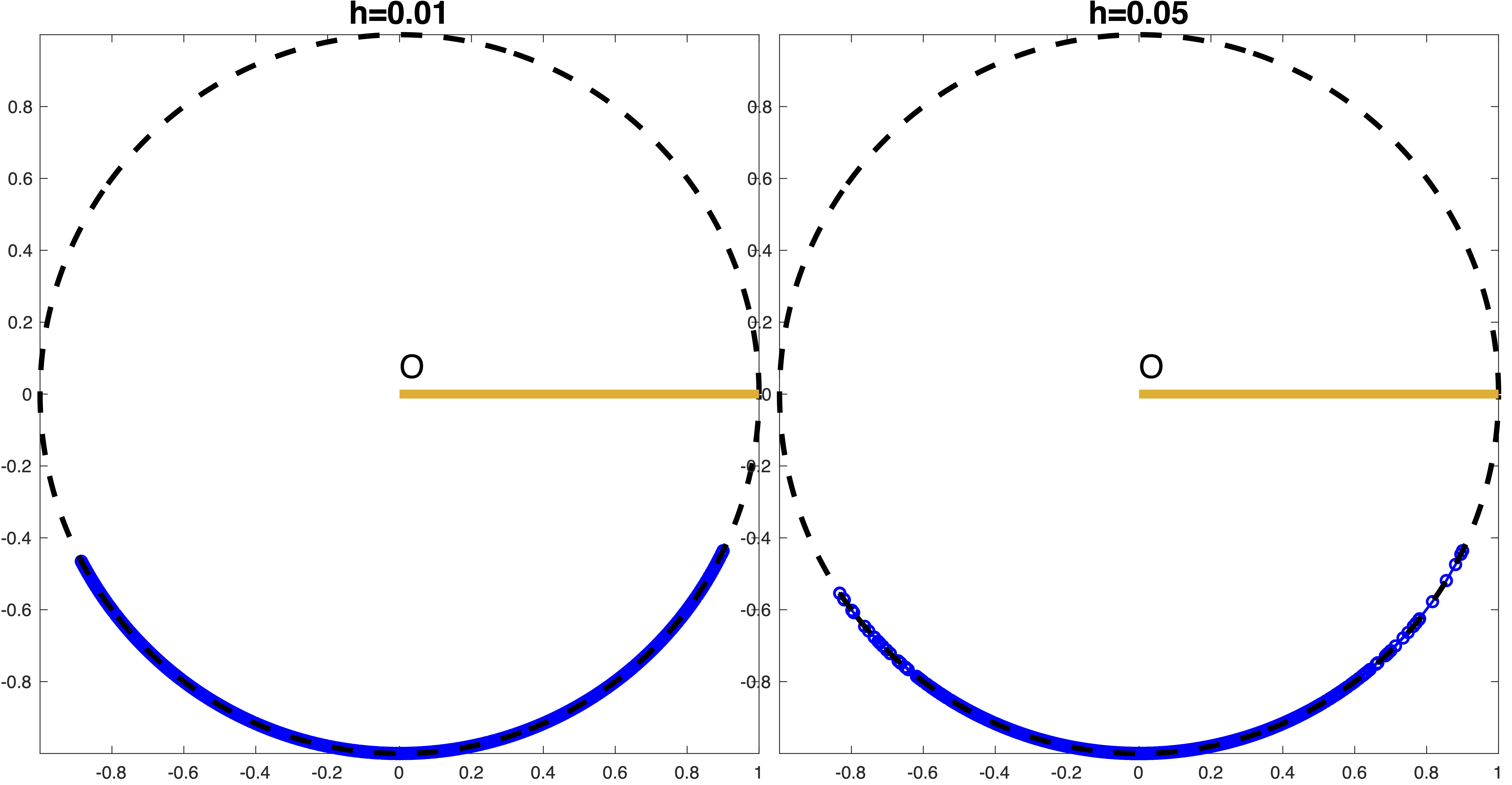
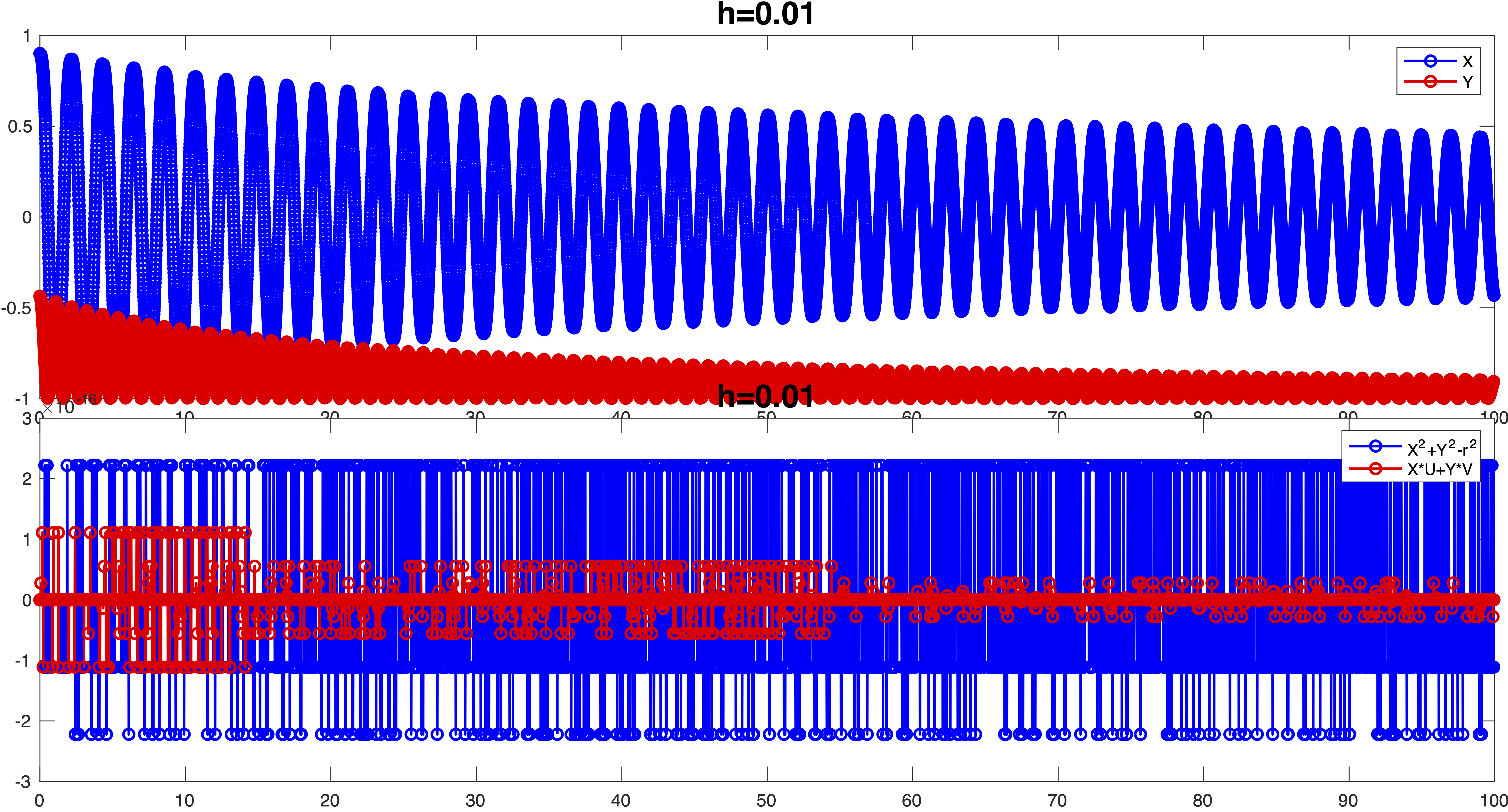
Fourth-Order Runge–Kutta
\begin{aligned} K_1 &= h u_k\quad & L_1 &= h \mu\left(x_k,u_k\right)x_k \\ K_2 &= h\left(u_k+\frac{L_1}{2}\right)\quad& L_2 &= h \mu\left(x_k+\frac{K_1}{2},u_k+\frac{L_1}{2}\right)\left(x_k+\frac{K_1}{2}\right) \\ K_3 &= h\left(u_k+\frac{L_2}{2}\right)\quad & L_3 &= h\mu\left(x_k+\frac{K_2}{2},u_k+\frac{L_2}{2}\right)\left(x_k+\frac{K_2}{2}\right) \\ K_4 &= h\left(u_k+L_3\right)\quad & L_4 &= h\mu\left(x_k+K_3,u_k+L_3\right)\left(x_k+K_3\right) \end{aligned}
\begin{aligned} x_{k+1} &= x_k + \frac{K_1+2K_2+2K_3+K_4}{6} \\ u_{k+1} &= u_k + \frac{L_1+2L_2+2L_3+L_4}{6} \end{aligned}
T_{\max} = 10, x(0)=0.9, u(0)=0. The remaining value y(0) = \sqrt{r^2-x(0)^2} and v(0)=-x(0)u(0)/y(0).
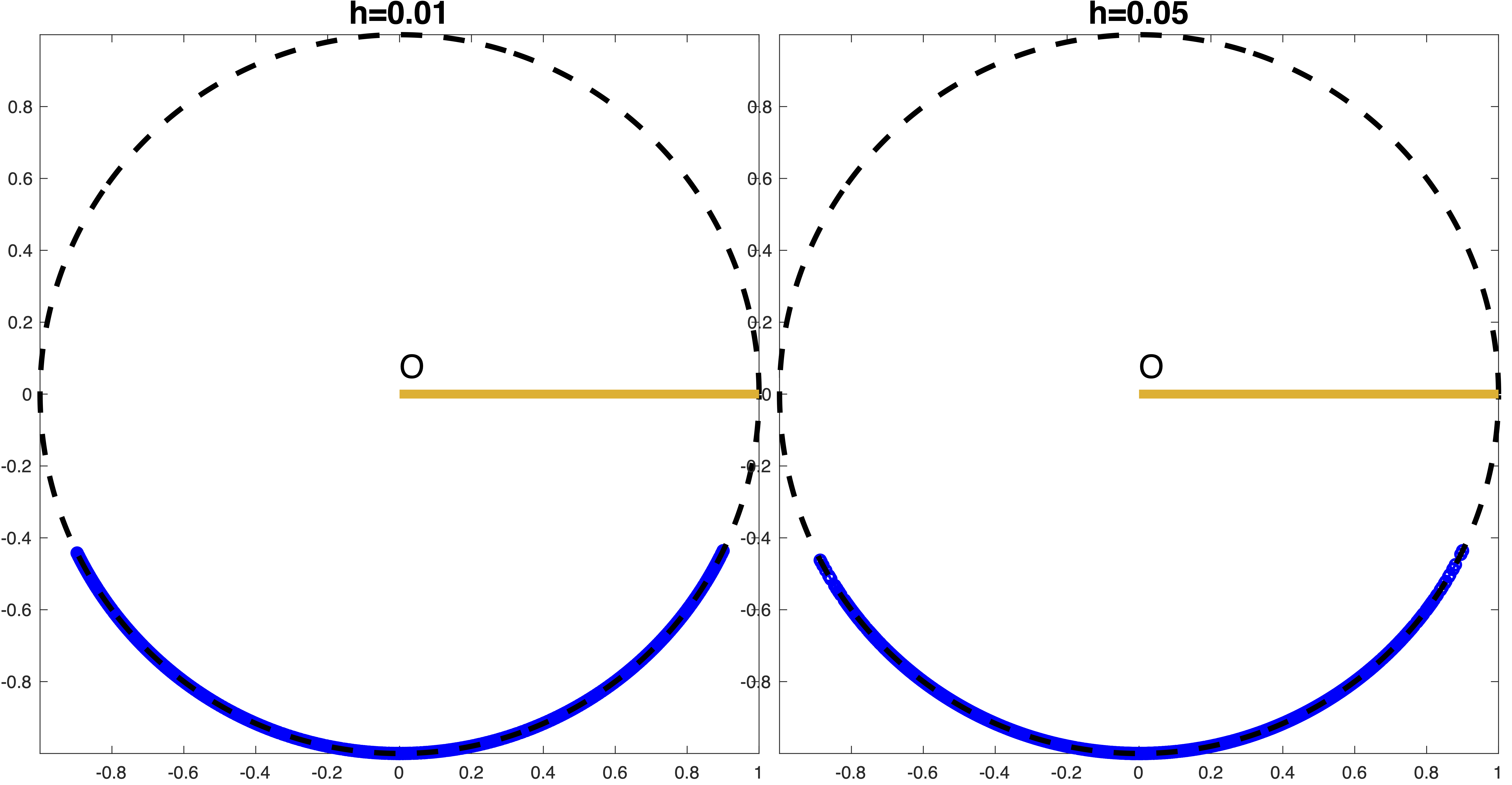
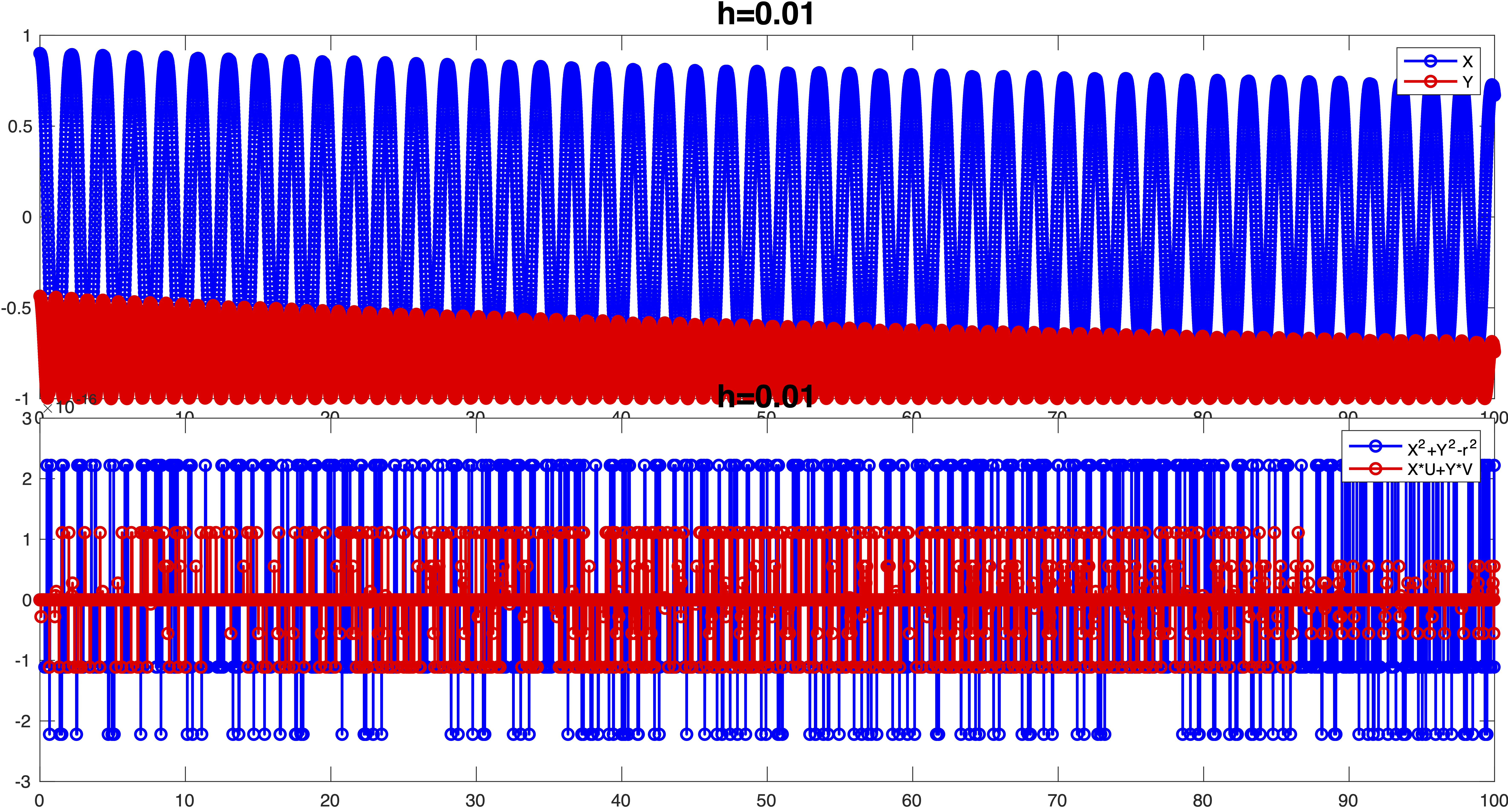
8.9 Order Reduction in DAE Integration
A time integrator of classical order p on ODEs can converge with a smaller order on a DAE. This order reduction is distinct from index reduction: index reduction changes the equations, whereas order reduction describes the observed convergence rate of a discretization.
Main mechanisms
Order reduction is most likely when
- algebraic or multiplier variables have a lower stage order than the differential variables;
- the DAE has index greater than one;
- the initial data satisfy the visible constraints but not all compatibility conditions;
- boundary data or external forcing are insufficiently smooth;
- a stiff transient makes the asymptotic error expansion nonuniform;
- projection or index reduction introduces an error larger than the local truncation error of the base method.
For Runge–Kutta methods, classical order alone is therefore not enough. Stage order and the method’s DAE-specific order conditions control how well the internal stages satisfy the constraints.
How to detect it
Run the same problem with h, h/2, and h/4 and estimate
p_{\rm obs} = \log_2\frac{\|\bm e_h\|}{\|\bm e_{h/2}\|}.
Measure errors separately for differential variables, algebraic variables, multipliers, and constraint residuals. A single combined norm can conceal that only one component has lost order. Repeat the experiment after tightening the nonlinear-solver tolerance so that iteration error is not mistaken for discretization error.
Mitigation
- Compute fully consistent initial values, including hidden constraints.
- Prefer methods designed for the DAE class, such as stiffly accurate implicit Runge–Kutta formulas or appropriate BDF methods.
- Reduce the index while retaining and monitoring all invariants.
- Match projection accuracy to the local error target of the time integrator.
- Use a start-up procedure of sufficient order after events or discontinuous inputs.
- Confirm the claimed order by a mesh-refinement table rather than by the solver’s status flag.
WarningWhat an adaptive controller sees
An ODE error estimator can control its own embedded difference while missing the dominant algebraic or constraint error. For a DAE, acceptance tests should include both the temporal error estimate and scaled constraint residuals.
8.10 Choosing a Numerical DAE Method
Method selection begins with structure, not with a solver name. The diagram summarizes a practical first decision; every branch still requires consistent initialization and residual monitoring.
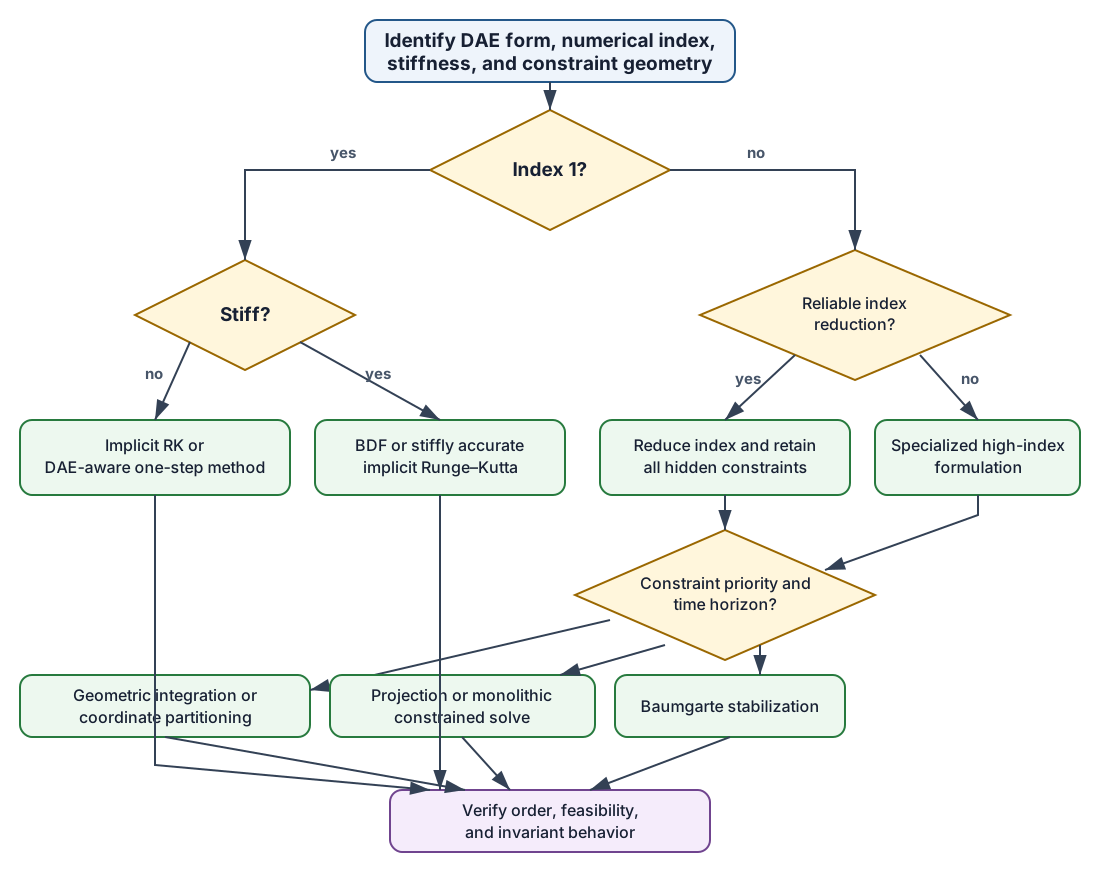 {#fig-dae-method-selection width=“100%”,bg=“white”}
Decision table
| Structure | Good first choice | Main check |
|---|---|---|
| index-1, non-stiff | implicit RK or Rosenbrock-type DAE method | local error and algebraic residual |
| index-1, stiff | BDF or L-stable implicit RK | nonlinear convergence and stiff decay |
| reducible high index | index reduction plus projection | hidden constraints and observed order |
| constrained mechanics, long time | SHAKE/RATTLE-type or partitioned geometric method | constraints, energy, momentum |
| moderate drift acceptable | Baumgarte stabilization | parameter sensitivity and artificial damping |
| exact pointwise feasibility | projection or monolithic constrained solve | projection conditioning |
| changing constraint rank | event handling and rank-revealing linear algebra | rank and consistency after events |
No branch removes the need for a convergence study. Stiffness, index, and constraint geometry can change along one trajectory, so production codes should expose diagnostics rather than silently switching interpretations.
8.11 Examples
An index-two Van der Pol oscillator
The Van der Pol equation x'' - \mu(1-x^2)x' + x = 0 represents a classic example of a nonlinear oscillator with nonlinear damping, widely used in the study of dynamical systems and electrical circuits.
Stiff DAE Form
To transform the equation into an index-2 DAE (Differential-Algebraic Equation) system @Mazzia2003, we introduce:
- The variable y = x' to obtain a first-order system
- An additional state z
The resulting DAE is: \left\{ \begin{aligned} x' &= y \\ y' &= \mu(1-x^2)y - x \\ 0 &= x^2 - z^2 + 5 \end{aligned} \right.
Semi-Explicit Form
For the previous DAE system introduce dummy variables y_{\text{dot}}, z_{\text{dot}} and the system decomposes into differential (blue) and algebraic (red) components:
\left\{ \color{blue} \begin{aligned} x' & = y\\ y' & = y_{\text{dot}} \\ z' & = z_{\text{dot}} \end{aligned} \right. \quad \bigoplus \quad \left\{ \color{DarkRed} \begin{aligned} 0 & = {\color{blue}y_{\text{dot}}} - \mu(1-x^2)y + x & \text{(Constraint 1)}\\ 0 & = x^2 - z^2 + 5& \text{(Constraint 2)} \end{aligned} \right.
For this DAE we have:
- Differential variables: x, y, z.
- Algebraic variables: y_{\text{dot}}, z_{\text{dot}}.
Reduction Procedure
We attempt to solve for y_{\text{dot}}, z_{\text{dot}}, but the system is not yet solvable explicitly. We proceed by differentiating.
Step 1: Differentiate algebraic constraints
We now differentiate the constraints to reduce the index. Here we want to differentiate only the algebraic equation that can reduce the index and do not introduce new differential equation. Here we want to avoid to introduce derivative of the algebraic variable unless is strictly necessary.
We construct a dependency table to identify which constraints to differentiate:
\begin{array}{c|cc} & y_{\text{dot}} & z_{\text{dot}} \\[0.5em] \hline \\[0.1em] \text{(Constraint 1)} & 1 & 0 \\[0.5em] \text{(Constraint 2)} & 0 & 0 \end{array}
a 0 means the the function do not depend on the variable on the column. A 1 means dependence. Last constraint is candidate for differentiation as it doesn’t introduce new algebraic variables. Differentiate thus the last constraints and substitute known variable in differential form using the ODE part
\text{(Constraint 2)}' = 2xx' - 2 z z' = 2 x y - 2 z z_{\text{dot}}
so that the DAE become:
\left\{ \color{blue} \begin{aligned} x' & = y\\ y' & = y_{\text{dot}} \\ z' & = z_{\text{dot}} \end{aligned} \right. \quad \bigoplus \quad \left\{ \color{DarkRed} \begin{aligned} 0 & = y_{\text{dot}} - \mu(1-x^2)y + x & \text{(Constraint 1)}\\ 0 & = 2 x y - 2 z z_{\text{dot}} & \text{(Constraint 2)}' \\[0.5em] \color{DarkGreen} 0 & \color{DarkGreen} = x^2 - z^2 + 5 & \color{DarkGreen}\text{(Constraint 2)}\\ \end{aligned} \right.
The red algebraic equations are the new algebraic equation after the derivation. The green algebraic equation is the hidden constraints that is removed from the DAE system but that is satisfied by choosing the right initial conditions.
The red part cannot determine the algebraic variable and must be differentiated again.
Step 2: Differentiate (again) the algebraic constraints
To find the right candidate(s) here we write a table of the dependencies \begin{array}{c|cc} & y_{\text{dot}} & z_{\text{dot}} \\[0.5em] \hline \\[0.1em] \text{(Constraint 1)} & 1 & 0 \\[0.5em] \text{(Constraint 2)}' & 0 & 1 \end{array}
The table shows that the nonlinear system is structurally non singular and algebraic constraints can be solved. From \text{(Constraint 2)}' solve for z_{\text{dot}} and from \text{(Constraint 1)} solve for y_{\text{dot}}
z_{\text{dot}} = \frac{xy}{z}, \qquad y_{\text{dot}} = \mu(1-x^2)y - x
ODE Form
Thus DAE now can be reduced to an ODE and can be written as:
\left\{ \color{blue} \begin{aligned} x' & = y\\ y' & = y_{\text{dot}} = \mu(1-x^2)y - x \\ z' & = z_{\text{dot}} = \frac{xy}{z} \end{aligned} \right. \quad \bigoplus \quad \color{DarkGreen} x^2 - z^2 + 5=0,\quad\text{(Constraint 1)}
Baumgarte Stabilization
Baumgarte stabilization is a classical technique used to prevent this drift. Instead of enforcing a constraint like:
z(t) = 0
we instead modify it to a differential equation:
\frac{dz}{dt} + \frac{1}{\tau} z = 0
This form ensures that any initial deviation from the constraint decays exponentially with a rate controlled by the parameter \tau. The smaller \tau is, the stronger the correction applied.
The exact solution is:
z(t) = z_0 \, e^{-t/\tau}
In the following example, we simulate the stabilized equation for different values of \tau and visualize how quickly the constraint error decays.
Impact of the stabilization parameter \tau.
The plot clearly shows the impact of the stabilization parameter \tau:
- Small \tau (e.g., 0.01): The solution quickly decays to zero, meaning constraint violations are rapidly corrected. However, this can introduce numerical stiffness.
- Large \tau (e.g., 5): The decay is slow, allowing more deviation from the constraint over time.
This trade-off is at the heart of Baumgarte stabilization: small \tau improves accuracy but increases stiffness and numerical cost, while large \tau is easier to integrate but less effective at controlling constraint drift.
In real DAE systems, choosing \tau often involves tuning based on system stiffness and desired constraint enforcement.
For this DAE the hidden constraints can be used to stabilize the algebraic constraint \text{(Constraint 1)}
\color{Olive}\text{(Constraint 1)}_{\text{stab}} = \text{(Constraint 1)}' + {\color{DarkOrange}\frac{1}{\tau}} \text{(Constraint 1)}= 0
and substituting (diving also by 2)
\color{Olive}\text{(Constraint 1)}_{\text{stab}} = x\,y-z\,z_{\text{dot}}+ {\color{DarkOrange}\frac{1}{\tau}}\frac{x^2-z^2+5}{2}
and using the stabilized constraints
\left\{ \color{blue} \begin{aligned} x' & = y\\ y' & = \mu(1-x^2)y - x \\ z' & = \frac{xy}{z}+{\color{DarkOrange}\frac{1}{\tau}\frac{x^2-z^2+5}{2z}} \end{aligned} \right. \quad \bigoplus \quad \color{DarkGreen} x^2 - z^2 + 5=0,\quad\text{(Constraint 1)}