Appendix A — Gaussian Elimination and Echelon Forms

This appendix collects the linear-algebra machinery used throughout the book, and in particular by the index-reduction algorithms of the DAE part. It is placed outside the main text because it is a prerequisite rather than a result: readers who are comfortable with rank-revealing elimination, echelon forms, and the effect of pivoting on conditioning can skip it and refer back only for notation.
Three facts are used repeatedly in the main text:
- any matrix, square or rectangular, singular or not, can be reduced to echelon form by elementary row operations (Theorem A.1);
- the reduction identifies a full-rank leading block and a zero block, which is exactly the separation between differential and algebraic equations in a DAE (Section 8.1);
- the numerical rank, and therefore that separation, depends on the pivoting strategy and on the conditioning of the matrix.
The Weierstrass canonical form is quite valuable from a theoretical standpoint. However, it can be computationally intensive since it necessitates the use of several Jordan canonical forms. In the following section, we will present a more numerically efficient algorithm for reducing a Differential Algebraic Equation (DAE) to an Ordinary Differential Equation (ODE). This method leverages the well-known Gaussian elimination technique, enhanced with differentiation to achieve the desired reduction.
A.1 Elimination Process
Before diving into DAE reduction to ODE, we will revisit some fundamental concepts and definitions that are pertinent to this process.
Definition A.1 Given a matrix
\bm{M} \in \mathbb{R}^{n \times m}
we define elementary operations as follows:
- Permutation of two rows (or columns),
- Linear combinations of rows (or columns).
These operations can also be viewed as specific forms of matrix multiplication.
Definition A.2 A non-singular matrix
\bm{P}_{[i,j]} \in \mathbb{R}^{n \times n}
is referred to as a permutation matrix (row or column depend on the application) if it is derived from the identity matrix \bm{I} \in \mathbb{R}^{n \times n} by swapping column i with column j.
Permutation matrices exhibit several noteworthy properties:
\bm{P}_{[i,j]}^{-1} = \bm{P}_{[i,j]}^{\intercal}: This shows that \bm{P}_{[i,j]} is an orthogonal matrix.
\bm{P}_{[i,j]}^{2} = \bm{I}: This indicates that \bm{P}_{[i,j]} is an involution matrix.
\bm{P}_{[i,j]}\bm{M}: This operation exchanges row i with row j.
\bm{M} \bm{P}_{[i,j]}: This operation exchanges column i with column j.
In a similar manner, we can define matrices that perform linear combinations of rows (or columns). These matrices are classified as elementary matrices.
Definition A.3 A matrix
\bm{F}_{[i,j]}(\alpha) \in \mathbb{R}^{n\times n}
is referred to as a row (or column) elementary matrix if it has the following structure:
\bm{F}_{[i,j]}(\alpha) = \begin{bmatrix} 1 & \dots & 0 & \dots & 0 & \dots & 0 \\ \vdots & \ddots & \vdots & & \vdots & & \vdots \\ 0 & \dots & 1 & & 0 & & 0 \\ \vdots & & \vdots & \ddots & \vdots & & \vdots \\ 0 & \dots & \alpha & \dots & 1 & \dots & 0 \\ \vdots & & \vdots & & \vdots & \ddots & \vdots \\ 0 & \dots & 0 & \dots & 0 & \dots & 1 \end{bmatrix}
where the (i,j) entry equals \alpha.
Remark A.1. An elementary matrix \bm{F}_{[i,j]}(\alpha) \in \mathbb{R}^{n\times n} is identical to the identity matrix of dimension n in all entries except for the (i,j) position, which is set to \alpha.
Elementary matrices have several key properties:
- The operation \bm{F}_{[i,j]}(\alpha) \bm{M} adds row j multiplied by \alpha to row i.
- The operation \bm{M} \bm{F}_{[i,j]}(\alpha) adds column i multiplied by \alpha to column j.
Theorem A.1 Rank normal form (Gaussian elimination with row and column operations).
Let \bm{M}\in\mathbb{R}^{n\times m} be a matrix of rank r (0\le r\le\min(n,m)). Then there exist invertible matrices \bm{L}\in\mathbb{R}^{n\times n} and \bm{R}\in\mathbb{R}^{m\times m} such that
\boxed{\bm{L}\bm{M}\bm{R}=\begin{bmatrix} \bm{I}_r & \bm{0}_{r\times(m-r)}\\ \bm{0}_{(n-r)\times r} & \bm{0}_{(n-r)\times(m-r)} \end{bmatrix}.}
In particular, by omitting the normalization of the pivots, \bm{I}_r may be replaced by an invertible diagonal matrix \bm{\Lambda}\in\mathbb{R}^{r\times r}. Empty blocks are understood when r=0, r=n, or r=m.
Proof. We prove the result constructively, using only elementary row and column operations. Each such operation is multiplication by an invertible matrix: row operations act on the left, column operations on the right.
Step 1: Choose a nonzero pivot
If \bm{M}=\bm{0}, then r=0 and the result holds with \bm{L}=\bm{I}_n and \bm{R}=\bm{I}_m. Otherwise, choose an entry M_{ij}\ne0. Exchange row i with row 1 and column j with column 1. The resulting matrix has the block form
\bm{M}_1=\begin{bmatrix} a & \bm{b}^{\mathsf T}\\ \bm{c} & \bm{D} \end{bmatrix},\qquad a\ne0,
where a is a scalar, \bm{b}\in\mathbb{R}^{m-1}, \bm{c}\in\mathbb{R}^{n-1}, and \bm{D}\in\mathbb{R}^{(n-1)\times(m-1)}.
Step 2: Eliminate the entries below and to the right of the pivot
For every i=2,\ldots,n, perform the row operation
R_i\longleftarrow R_i-\frac{(\bm{M}_1)_{i1}}{a}R_1.
This eliminates the entries below a and gives
\begin{bmatrix} a & \bm{b}^{\mathsf T}\\ \bm{0} & \bm{D}-\dfrac{\bm{c}\bm{b}^{\mathsf T}}{a} \end{bmatrix}.
Next, for every j=2,\ldots,m, perform the column operation
C_j\longleftarrow C_j-\frac{b_{j-1}}{a}C_1.
We obtain
\bm{M}_2=\begin{bmatrix} a & \bm{0}\\ \bm{0} & \bm{S} \end{bmatrix},\qquad \bm{S}=\bm{D}-\frac{\bm{c}\bm{b}^{\mathsf T}}{a}.
The matrix \bm{S} is the Schur complement of the pivot a. Because the operations are invertible, they preserve rank. Hence
\operatorname{rank}(\bm{M}) =\operatorname{rank}(\bm{M}_2) =1+\operatorname{rank}(\bm{S}),
so \operatorname{rank}(\bm{S})=r-1.
Step 3: Repeat on the remaining submatrix
Apply the same procedure to \bm{S}, without modifying the already eliminated first row and column. At each step, a nonzero pivot is isolated and the rank of the remaining submatrix decreases by one.
After exactly r nonzero pivots, the remaining submatrix has rank zero and is therefore the zero matrix. We obtain
\bm{L}_0\bm{M}\bm{R}_0= \begin{bmatrix} \bm{\Lambda} & \bm{0}\\ \bm{0} & \bm{0} \end{bmatrix},\qquad \bm{\Lambda}=\operatorname{diag}(a_1,\ldots,a_r),\quad a_k\ne0.
Step 4: Normalize the pivots
Multiply the first r rows by 1/a_1,\ldots,1/a_r, respectively. In matrix form, use the invertible diagonal matrix
\bm{D}_0=\operatorname{diag}(a_1^{-1},\ldots,a_r^{-1}, \underbrace{1,\ldots,1}_{n-r}).
Then, setting \bm{L}=\bm{D}_0\bm{L}_0 and \bm{R}=\bm{R}_0,
\bm{L}\bm{M}\bm{R}= \begin{bmatrix}\bm{I}_r&\bm{0}\\\bm{0}&\bm{0}\end{bmatrix}.
All the matrices used to construct \bm{L} and \bm{R} are invertible (permutations, additions of multiples of rows or columns, and nonzero scalings). Their products are therefore invertible, as required.
To illustrate the algorithm clearly, we provide the following example.
A.2 Echelon Form
A matrix is in row echelon form if:
All nonzero rows are above rows of all zeros.
Each leading entry (first nonzero number from the left) of a row is strictly to the right of the leading entry of the row above it.
All entries in a column below a leading entry are zeros.
Example of a matrix in row echelon form:
\begin{bmatrix} \color{magenta}1 & \color{magenta}2 & \color{magenta}0 & \color{magenta}3 \\ 0 & \color{magenta}4 & \color{magenta}1 & \color{magenta}5 \\ 0 & 0 & 0 & \color{magenta}6 \\ 0 & 0 & 0 & 0 \end{bmatrix}
Another example of a matrix in row echelon form:
\begin{bmatrix} \color{magenta}1 & \color{magenta}2 & \color{magenta}3 \\ 0 & \color{magenta}4 & \color{magenta}0 \\ 0 & 0 & \color{magenta}6 \end{bmatrix}
Elementary Row Operations
To transform a matrix into echelon form, we use three elementary row operations, each of which corresponds to multiplying on the left by an elementary matrix:
Swapping two rows \Rightarrow Multiply by a permutation matrix.
Multiplying a row by a nonzero scalar \Rightarrow Multiply by a diagonal matrix.
Adding or subtracting a multiple of one row to another row \Rightarrow Multiply by a lower triangular matrix.
Each elementary matrix is obtained by applying the corresponding row operation to the identity matrix.
Reduction Procedure
Step 1: Identify the Leftmost Nonzero Column (Pivot Column)
Scan the columns from left to right to find the first column that contains a nonzero entry.
The first nonzero number in that column will be our pivot.
Step 2: Ensure the Pivot is in the First Row of the Submatrix
If necessary, swap rows to move a row with a nonzero pivot to the top.
This corresponds to multiplying by a permutation matrix P.
Step 3: Zero Out All Entries Below the Pivot
For each row below the pivot row, subtract an appropriate multiple of the pivot row to make the entries below the pivot zero.
This operation is equivalent to multiplying by a lower triangular elementary matrix L.
Step 4: Normalize the Pivot (Optional but Useful)
The pivot can be scaled to 1 by dividing the row by the pivot value.
This step is equivalent to multiplying by a diagonal matrix \bm{D}.
Step 5: Move to the Next Column and Repeat
Find the next pivot column (to the right of the current pivot).
Repeat Steps 2-4 for the remaining sub-matrix.
Continue this process until all pivot positions are correctly set.
At each step, the transformation can be written as:
\bm{L}_k \bm{D}_k \bm{P}_k \cdots \bm{L}_2 \bm{D}_2 \bm{P}_2 \bm{L}_1 \bm{D}_1 \bm{P}_1 \bm{A} = \bm{U}
where \bm{U} is the echelon form of \bm{A}, and the matrices \bm{P}, \bm{D}, \bm{L} represent elementary row operations.
Echelon-Form Example
Given the matrix:
\bm{A} = \begin{bmatrix} 2 & 4 & 6 \\ 1 & 3 & 5 \\ 3 & 7 & 8 \end{bmatrix}
Step 1: Make the First Pivot 1
Swap row 1 and row 2 using permutation matrix \bm{P}:
\bm{P}\bm{A} = \begin{bmatrix} 1 & 3 & 5 \\ 2 & 4 & 6 \\ 3 & 7 & 8 \end{bmatrix}
Step 2: Zero Out Below the Pivot
Subtract 2 times row 1 from row 2 and 3 times row 1 from row 3 using lower triangular matrix \bm{L}_1:
\bm{L}_1 \bm{P} \bm{A} = \begin{bmatrix} 1 & 3 & 5 \\ 0 & -2 & -4 \\ 0 & -2 & -7 \end{bmatrix}
Step 3: Normalize the Second Pivot
Multiply row 2 by -\frac{1}{2} using diagonal matrix \bm{D}_1:
\bm{D}_1 \bm{L}_1 \bm{P} \bm{A} = \begin{bmatrix} 1 & 3 & 5 \\ 0 & 1 & 2 \\ 0 & -2 & -7 \end{bmatrix}
Step 4: Zero Out Below the New Pivot
Add 2 times row 2 to row 3 using lower triangular matrix \bm{L}_2:
\bm{L}_2 \bm{D}_1 \bm{L}_1 \bm{P} \bm{A} = \begin{bmatrix} \color{magenta}1 & \color{magenta}3 & \color{magenta}5 \\ 0 & \color{magenta}1 & \color{magenta}2 \\ 0 & 0 & \color{magenta}-3 \end{bmatrix}
This matrix is now in row echelon form.
Singular-Matrix Example
Consider the singular matrix:
\bm{A} = \begin{bmatrix} 2 & 4 & 6 \\ 1 & 2 & 3 \\ 3 & 6 & 9 \end{bmatrix}
Step 1: Normalize the First Pivot
Swap row 1 and row 2:
\bm{P} \bm{A} = \begin{bmatrix} 1 & 2 & 3 \\ 2 & 4 & 6 \\ 3 & 6 & 9 \end{bmatrix}
Step 2: Zero Out Below the Pivot
Subtract 2 times row 1 from row 2 and 3 times row 1 from row 3:
\bm{L}_1 \bm{P} \bm{A} = \begin{bmatrix} \color{magenta}1 & \color{magenta}2 & \color{magenta}3 \\ 0 & 0 & 0 \\ 0 & 0 & 0 \end{bmatrix}
Since the last two rows are all zeros, the rank of the matrix is 1, meaning:
- The matrix has linearly dependent rows.
- The determinant is zero, confirming singularity.
- The system \bm{A}\bm{x} = \bm{b} may have either infinitely many solutions or no solution, depending on b.
Thus, the matrix does not have an inverse.
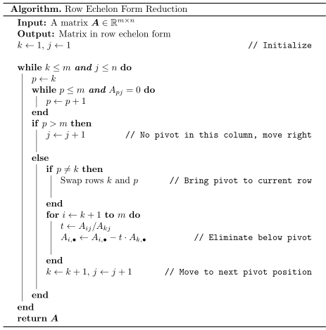
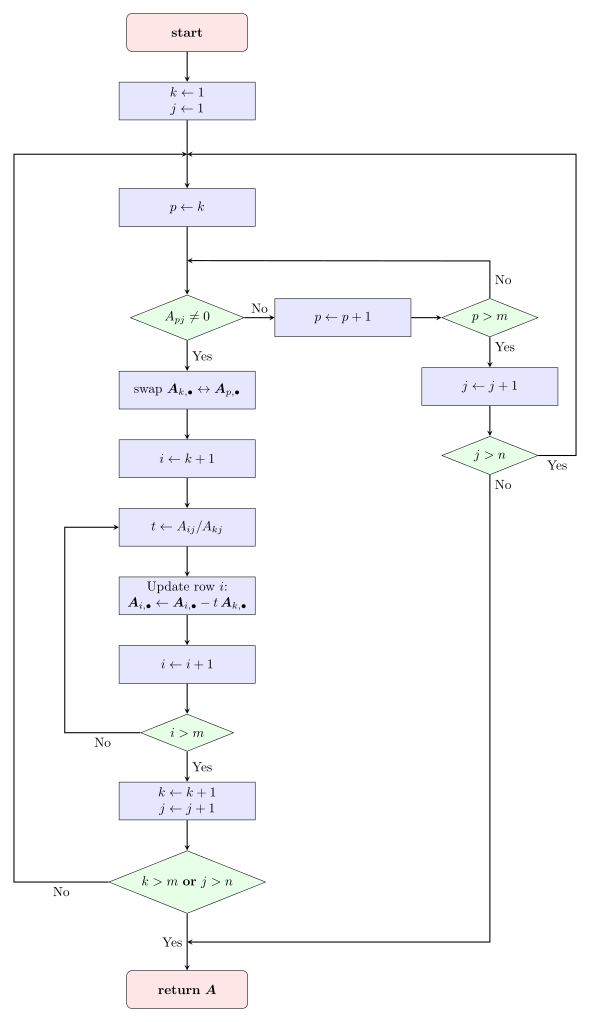
Reduction Algorithm
To transform a matrix into row echelon form:
- Identify the leftmost pivot column.
- Swap rows if necessary to bring a nonzero pivot to the top \bm{P}\bm{A}.
- Zero out all entries below the pivot \bm{L}_1, \bm{L}_2, \ldots.
- Normalize pivots if needed \bm{D}_1, \bm{D}_2, \ldots.
- Move to the next pivot column and repeat.
- Continue until all pivots are set correctly.
Each row operation corresponds to multiplication by an elementary matrix, leading to the factorization:
\bm{E}_k \cdots \bm{E}_2 \bm{E}_1 \bm{A} = \bm{U}
where \bm{U} is in echelon form, and \bm{E}_i are elementary matrices.
This method is a systematic approach to solving linear systems, computing ranks, and checking singularity conditions.
A.3 Equivalence transformations for a linear DAE
Consider \bm E\dot{\bm x}+\bm A\bm x=\bm f(t). Multiplication by a constant invertible matrix \bm P preserves its solution set:
\bm P\bm E\dot{\bm x}+\bm P\bm A\bm x=\bm P\bm f.
Column operations require a matching change of variables \bm x=\bm Q\bm z, with \bm Q constant and invertible:
(\bm P\bm E\bm Q)\dot{\bm z}+(\bm P\bm A\bm Q)\bm z=\bm P\bm f.
These are strict equivalence transformations of the pencil. Applying column operations to \bm E without transforming \bm A and the state does not preserve the DAE. If \bm Q=\bm Q(t) depends on time, an additional term \bm P\bm E\dot{\bm Q}\bm z appears.
A.4 Numerical rank, pivoting, and conditioning
Gaussian elimination with partial pivoting is preferable to unpivoted elimination for floating-point computations. Rank decisions require a scale-dependent tolerance: a tiny pivot is not a proof of exact singularity. For example,
\bm M_\varepsilon=\begin{bmatrix}1&1\\1&1+\varepsilon\end{bmatrix}, \qquad \det\bm M_\varepsilon=\varepsilon.
For every nonzero \varepsilon this matrix has exact rank two, but when |\varepsilon| is comparable with rounding error its numerical rank can be one. Rank-revealing QR with column pivoting or SVD can be more reliable than plain elimination, particularly when estimating the DAE index. In the SVD, singular values below a threshold of the form \tau\approx \max(m,n)\epsilon_{\mathrm{mach}}\sigma_{\max} are often classified as numerically zero; the correct threshold remains problem-dependent.
Important distinction: Gaussian elimination is an algebraic tool; differentiating a constraint changes the regularity requirements on the forcing and must not be confused with an invertible row operation. A differentiated system must retain the original undifferentiated constraints to preserve equivalence.