4 Inequality Constraints and KKT Conditions

4.1 Inequality Constraints
Let’s introduce now the problem of minimizing a function f(\bm{x}):\mathbb{R}^n\rightarrow \mathbb{R} considering a set of p inequality constraints in the form g_k(\bm{x}) \geq 0.
\begin{aligned} \text{minimize:} \qquad & f(\bm{x}) \\ \text{subject to:}\qquad & g_k(\bm{x}) \geq 0 \qquad k = 1,\dots,p \end{aligned}
Throughout this section, as in the preceding chapters, gradients of scalar-valued functions are row vectors. Thus \nabla g_k(\bm x)\bm d is the directional derivative of g_k along the column direction \bm d.
The first approach to this problem is by trying to transform the inequality constraints g_k into equality constraints (so having h_k(\bm{x}) = 0). This can be done considering that each constraint can be expressed as
g_k(\bm{x}) = \varepsilon_k^2 \geq 0 \quad \implies \quad h_k(\bm{x},\varepsilon_k) = g_k(\bm{x}) - \varepsilon_k^2 = 0
Doing this process for each constraint we can determine a minimization problem that depends both on the function variable \bm{x} but also on the so called slack variables \bm{\varepsilon}:
\begin{aligned} \text{minimize:} \qquad & f(\bm{x}) \\ \text{subject to:}\qquad & h_k(\bm{x}, \bm{\varepsilon}) = 0 \qquad k = 1,\dots,p \end{aligned}
This kind of problem increases the computational costs because it increases the number of optimization variables from n to n+p.
We used the expression \varepsilon_k^2 and not \varepsilon_k because with this expression we don’t need to specify one more inequality \varepsilon_k \geq 0.
Example 4.1 Let’s consider the following problem:
\begin{aligned} \text{minimize:} \qquad & f(x,y) = x^2 \\ \text{subject to:}\qquad & x^2+y^2\leq 1 \\ & x+y \geq 0 \end{aligned}
In order to solve this problem we have to reduce the inequality constraints to equality constraints; considering the first constraint, that has to be expressed in the form g_1(x,y) \geq 0 and so
\begin{aligned} g_1(x,y) & = 1 -x^2-y^2 \geq 0 \\ & \Downarrow \\ h_1(x,y,\varepsilon_1) & = 1-x^2-y^2-\varepsilon_1^2 \end{aligned}
In the same way it’s possible to express the second inequality as the a constraint
h_2(x,y,\varepsilon_2) = x+y-\varepsilon_2^2
With this expression being set the problem reduces to the form
\begin{aligned} \text{minimize:} \qquad & f(x,y,\epsilon_1,\epsilon_2) = x^2 \\ \text{subject to:}\qquad & h_1(x,y,\epsilon_1,\epsilon_2) = 1- x^2 - y^2 - \epsilon_1^2 = 0 \\ & h_2(x,y,\epsilon_1,\epsilon_2) = x+y - \varepsilon_2^2 = 0 \end{aligned}
With the problem stated in this way we can build the Lagrangian that depends on both the original variables x,y but also the slack variables \epsilon_1,\epsilon_2 and so
\begin{aligned} \mathcal{L}(\underbrace{x,y,\epsilon_1,\epsilon_2}_{\bm{x}},\underbrace{\lambda_1,\lambda_2}_{\bm{\lambda}}) &= f(\bm{x}) - \lambda_1 h_1(\bm{x}) - \lambda_2 h_2(\bm{x}) \\ & = x^2 - \lambda_1 \big( 1- x^2-y^2-\epsilon_1^2 \big) - \lambda_2 \big( x+y-\epsilon_2^2 \big) \end{aligned}
To find the local minimum point we can start using the first necessary condition of the Lagrangian multiplier, so by determining all the stationary points such that \nabla \mathcal{L} = \bm{0}; in practice this means solving the following nonlinear system of 6 equations in 6 variables:
\left\{ \begin{aligned} \partial/\partial_x \mathcal{L}:&& 2x +2\lambda_1x -\lambda_2 &= 0 \\ \partial/\partial_y \mathcal{L} :&& 2\lambda_1 y - \lambda_2 &= 0\\ \partial/\partial_{\epsilon_1}\mathcal{L} :&& 2\lambda_1\epsilon_1 &= 0 \\ \partial/\partial_{\epsilon_2}\mathcal{L} :&& 2\lambda_2 \epsilon_2 &= 0 \\ \partial/\partial_{\lambda_1} \mathcal{L} :&& x^2+y^2 + \epsilon_1^2-1 &= 0 \\ \partial/\partial_{\lambda_2}\mathcal{L} :&& x + y - \epsilon_2^2 &= 0 \end{aligned} \right.
Solving minimization problems with inequality constraints can be tricky using the Lagrangian multiplier method and so other algorithm (like the KKT that’s going to be explained) are usually preferred. However this kind of system can be solved by cases; considering in fact the second and third equations we can discriminate the solution considering the various combination when \epsilon_1, \epsilon_2 are equal (or not) to zero.
A direct case analysis is possible, but this reformulation also shows an important drawback of squared slack variables: when an inequality is active, the corresponding slack variable is zero and the gradient of the equality constraint with respect to that slack variable vanishes. Therefore the usual equality-constraint regularity assumptions may fail exactly at active inequalities.
For this example the global minimum value is immediately seen to be
f_{\min}=0,
because f(x,y)=x^2\geq0. It is attained at every feasible point with x=0. The constraints then give
y^2\leq1,\qquad y\geq0,
hence the complete set of minimizers is
\boxed{(x,y)=(0,y),\qquad y\in[0,1].}
The slack-variable formulation reproduces these points with
\epsilon_1^2=1-y^2,\qquad \epsilon_2^2=y.
However, KKT conditions applied directly to the inequalities are cleaner and avoid the artificial degeneracy introduced by squared slack variables.
Statement of the KKT conditions
The Karush-Kuhn-Tucker (KKT) conditions provide first-order necessary conditions for local optimality under a constraint qualification, and, with additional second-order assumptions, sufficient conditions for strict local optimality. They are used to analyze whether a point \bm{x}^\star is a minimum point of a minimization problem subject to equality and inequality constraints, so for the problem
\begin{aligned} \text{minimize:} \qquad & f(\bm{x}) \\ \text{subject to:}\qquad \ & h_k(\bm{x}) = 0 \qquad && k=1,\dots, m\\ & g_k(\bm{x}) \geq 0 &&k = 1,\dots,p \end{aligned}
where f,h_k,g_k: \mathbb{R}^n\rightarrow \mathbb{R} are real-valued functions.
To state these conditions, define the set of active inequality constraints \mathcal{A} as
\mathcal{A}(\bm{x}^\star) = \big\{ k \ | \ g_k(\bm{x}^\star) = 0 \big\}
An inequality is active at \bm{x}^\star when it holds with equality, i.e. when the point lies on the corresponding constraint boundary.
Qualified constraints
Given \bm g:\mathbb R^n\to\mathbb R^p and \bm h:\mathbb R^n\to\mathbb R^m, with components of class C^1, the Linear Independence Constraint Qualification (LICQ) holds at a feasible point \bm{x}^\star if
\big\{ \nabla g_k(\bm{x}^\star) : k\in\mathcal A(\bm{x}^\star) \big\} \cup \big\{ \nabla h_j(\bm{x}^\star) : j=1,\ldots,m \big\}
is a linearly independent set. Equivalently, the Jacobian obtained by stacking the equality-constraint gradients and the active inequality-constraint gradients has full row rank.
LICQ is a convenient constraint qualification, but it is stronger than necessary for first-order KKT conditions; weaker qualifications such as MFCQ can also be used.
Example 4.2 (qualification of a point) Considering the minimization problem started in example Example 2.2 stated as
\begin{aligned} \text{minimize:} \qquad & f(x,y,z) = x - y + z^2 \\ \text{subject to:} \qquad & h_1(x,y,z) = x^2 + y^2 - 2 = 0 \\ & h_2(x,y,z) = x+z-1 = 0 \end{aligned}
and considering the candidate point of minimum (resulting from the solution of the non-linear system)
\begin{aligned} x^\star &= \frac{\sqrt 3}{2} - \frac{1}{2}\\ y^\star &= \frac 1 2 + \frac{\sqrt 3}{2} \\ z^\star &= \frac 3 2 - \frac{\sqrt 3}{2} \\ \lambda_1^\star & = \frac{1}{2} - \frac{\sqrt3}{2} \\ \lambda_2^\star &= 3-\sqrt{3} \end{aligned}
In order to check if the chosen point is qualified it’s necessary to check if the gradients of the equality constraint and the active ones (that in this case are not present because there aren’t inequality constraints) are linearly independent. In order to solve this problem first we need to build the matrix H represent the gradients of the constraints:
H(x,y,z) = \begin{bmatrix} \nabla h_1(x,y,z) \\ \nabla h_2(x,y,z) \end{bmatrix} = \begin{bmatrix} 2x & 2y & 0 \\ 1 & 0 & 1 \end{bmatrix}
\implies \qquad H^\star= H(x^\star,y^\star,z^\star) = \begin{bmatrix} \sqrt 3 - 1 & 1 + \sqrt 3 & 0 \\ 1 & 0 & 1 \end{bmatrix}
It’s straightforward to see that the lines of the matrix H^\star are linearly independent, considering in fact the rank of H^\star by analysing the columns we see that’s equal to 2, so equalizing the number of the constraints.
KKT first order necessary condition
Let f\in C^1(\mathbb{R}^n) a function to minimize subject to the inequality
\bm{g}\in C^1(\mathbb{R}^n,\mathbb{R}^p)
and equality
\bm{h} \in C^1(\mathbb{R}^n,\mathbb{R}^m)
constraint maps. If \bm{x}^\star is a local minimizer and LICQ holds at \bm{x}^\star, then there exist multipliers \bm{\lambda}^\star\in\mathbb{R}^m and \bm{\mu}^\star\in\mathbb{R}^p such that the following KKT conditions hold:
\begin{aligned} \nabla_{\bm{x}} \mathcal{L} \big(\bm{x}^\star,\bm{\lambda}^\star,\bm{\mu}^\star\big) & = \bm{0} \\ h_k\big(\bm{x}^\star\big) & = 0 \qquad && k = 1,\dots,m\\ g_k\big(\bm{x}^\star\big) & \geq 0 && k = 1,\dots,p \\ \mu_k^\star g_k\big(\bm{x}^\star\big) & = 0 && k = 1,\dots,p \\ \mu_k^\star & \geq 0 && k = 1,\dots,p \end{aligned} \tag{4.1}
These are, respectively, stationarity, primal feasibility, complementary slackness, and dual feasibility. With the convention g_k(\bm{x})\geq0 and \mathcal L=f-\sum_k\mu_k g_k-\sum_j\lambda_jh_j, the correct sign is \mu_k\geq0.
where the Lagrangian is in this case defined as
\mathcal{L}(\bm{x},\bm{\lambda},\bm{\mu}) = f(\bm{x}) - \sum_{k=1}^p \mu_k g_k(\bm{x}) - \sum_{k=1}^m \lambda_k h_k(\bm{x})
Example 4.3 Solving minimization problem with the KKT conditions is generally easier; considering the case of the minimization problem in Example 4.1 the Lagrangian will depend only on 4 parameters (instead of 6 as in that example):
\mathcal{L}(x,y,\mu_1,\mu_2) = x^2 - \mu_1\big(1-x^2-y^2\big) - \mu_2\big(x+y\big)
Using the first-order KKT conditions, the stationarity and complementarity equations are
\left\{\begin{aligned} \left.\begin{aligned} 2x +2\mu_1x - \mu_2 &= 0 \\ 2 \mu_1 y - \mu_2 &= 0 \end{aligned} \right\} & \quad \nabla_{\bm{x}} \mathcal{L}\big(\bm{x}, \bm{\lambda}\big) \\ \left. \begin{aligned} \mu_1\big(1-x^2-y^2\big) & = 0 \\ \mu_2 \big(x+y\big) & = 0 \end{aligned} \right\} & \quad \mu_k g_k\big(\bm{x} \big) = 0\\ \mu_1,\mu_2 \geq 0 \quad & \end{aligned} \right.
These equations must be considered together with primal feasibility 1-x^2-y^2\ge0, x+y\ge0 and dual feasibility \mu_1,\mu_2\ge0. The system can then be solved by cases:
If \mu_1 = \mu_2 = 0 then the last two equalities are always verified, while the first two becomes
\begin{cases} 2x = 0 \\ 0 = 0 \end{cases} this means that x = 0, while y is a free parameter that must satisfy both the constraints x+y\geq 0 (so that y \geq 0) and 1-x^2-y^2 \geq 0 (and so 1-y^2 \geq 0 that determines -1 \leq y \leq 1): considering both condition at the same time we have that \begin{aligned} & \begin{cases} y \geq 0 \\ -1 \leq y \leq 1 \end{cases} \quad \implies \quad \\[0.5em] & \text{solution: } x = \mu_1 = \mu_2 = 0 \quad y \in [0,1] \end{aligned}
When considering \mu_1 \neq 0 and \mu_2 = 0 the system of equations become \begin{cases} 2x + 2 \mu_1x = 0 \\ 2\mu_1 y = 0 \\ \mu_1\big(1-x^2-y^2\big) = 0 \end{cases} Based on the assumption of the value \mu_1, from the second equation we determine that y must be equal to 0 and so the third equation becomes 1-x^2 = 0 whose solutions are \pm 1. Considering that the first equation can be factorised as 2x(1+\mu_1) = 0 (and x\neq 0), then in order to satisfy the relation \mu_1 must be -1, but this imply that \mu_1 is negative and it’s an unacceptable solution, so for \mu_1 \neq 0,\mu_2=0 no solutions of the system can be found;
Considering instead \mu_1 = 0 and \mu_2 \neq 0 the system becomes \begin{cases} 2x - \mu_2 = 0 \\ -\mu_2 = 0 \\ \mu_2(x+y) = 0 \end{cases} The second equation states that \mu_2 must be equal to 0 and so the solution of this problem is the same as the first case considered;
Considering both variables \mu_1,\mu_2 \neq 0 we have to solve the full systems; considering the last two equations we have that \begin{aligned} & \begin{cases} x+y = 0 \\ 1-x^2-y^2 = 0 \end{cases} \\ & \implies\quad x = -y \\ & \implies\quad 1-2x^2 = 0 \end{aligned} and so it means that the two possible solution for the systems are (x,y) = \left( \pm \frac{1}{\sqrt{2}}, \mp \frac{1}{\sqrt{2}} \right). Considering the first case where x = 1/\sqrt 2 the first two equations become \begin{aligned} & \begin{cases} \frac{2}{\sqrt 2} (1+\mu_1) - \mu_2 = 0 \\ -\frac 2 {\sqrt 2} \mu_1 - \mu_2 = 0 \end{cases} \\ & \implies \quad \mu_2 = - \frac 2 {\sqrt 2} \mu_1 \\ & \implies \quad \frac{4}{\sqrt 2} \mu_1 + \frac{2}{\sqrt 2} = 0 \\ & \implies \quad \mu_1 = - \frac{1}{2} \qquad \mu_2 = \frac{1}{\sqrt{2}} \end{aligned} In this case \mu_1 < 0 is an unacceptable solution of the problem, and also considering the point x = -1/\sqrt{2} the system becomes with no considerable solutions \begin{aligned} & \begin{cases} -\frac{2}{\sqrt 2} (1+\mu_1) - \mu_2 = 0 \\ \frac{2}{\sqrt 2} \mu_1 - \mu_2 = 0 \end{cases} \\ & \implies \quad \mu_1 = -\frac{1}{2}\quad \mu_2 = - \frac{1}{\sqrt{2}} \end{aligned}
The KKT solutions are therefore
(x,y)=(0,k),\qquad k\in[0,1].
In this example no second-order argument is actually needed to establish optimality: f(x,y)=x^2\ge0 everywhere, and every point above has f=0. Hence these points are exactly the global minimizers.
KKT second order necessary conditions
Assume now that f, h_k and g_k are of class C^2. Let \bm{x}^\star be a local minimizer at which LICQ holds, and let (\bm{\lambda}^\star,\bm{\mu}^\star) be the KKT multipliers.
The relevant set of first-order feasible directions is the critical cone
\mathcal C(\bm{x}^\star,\bm{\mu}^\star) = \left\{\bm z:\begin{array}{ll} \nabla h_j(\bm{x}^\star)\bm z=0, & j=1,\ldots,m,\\[0.2em] \nabla g_k(\bm{x}^\star)\bm z=0, & k\in\mathcal A(\bm{x}^\star),\ \mu_k^\star>0,\\[0.2em] \nabla g_k(\bm{x}^\star)\bm z\ge0, & k\in\mathcal A(\bm{x}^\star),\ \mu_k^\star=0. \end{array}\right\}.
Then the second-order necessary condition is
\boxed{ \bm z^T\nabla_{\bm x\bm x}^2\mathcal L (\bm{x}^\star,\bm{\lambda}^\star,\bm{\mu}^\star)\bm z\ge0 \qquad \forall\bm z\in\mathcal C(\bm{x}^\star,\bm{\mu}^\star). } \tag{4.2}
A simpler but weaker necessary test is obtained by restricting to the smaller subspace
\nabla h_j(\bm{x}^\star)\bm z=0, \qquad \nabla g_k(\bm{x}^\star)\bm z=0 \quad\forall k\in\mathcal A(\bm{x}^\star).
If the Hessian is negative in one of these directions, the candidate cannot be a local minimum. Passing this weaker test, however, does not establish local minimality.
For second-order sufficiency, one must test the whole critical cone. Replacing the inequality condition for active constraints with zero makes the set of directions smaller and is therefore not a valid sufficient test in general.
Consider the problem
\begin{aligned} \min_{x,y}\quad & f(x,y)=-x^2+y^2,\\ \text{subject to}\quad & g(x,y)=x\ge0. \end{aligned}
At the feasible point
(x^\star,y^\star)=(0,0),
the inequality is active. With the convention
\mathcal L(x,y,\mu)=f(x,y)-\mu g(x,y), \qquad \mu\ge0,
the stationarity condition is
\nabla f(0,0)-\mu^\star\nabla g(0,0)=0.
Since
\nabla f(0,0)=\begin{bmatrix}0&0\end{bmatrix}, \qquad \nabla g(0,0)=\begin{bmatrix}1&0\end{bmatrix},
we obtain
\mu^\star=0.
If one incorrectly treats the active inequality as an equality, one tests only the kernel
\mathcal K = \left\{z:\nabla g(0,0)z=0\right\} = \left\{ \begin{bmatrix}0\\z_2\end{bmatrix}:z_2\in\mathbb R \right\}.
The Lagrangian Hessian is
\nabla^2_{xx}\mathcal L(0,0,0) = \begin{bmatrix} -2&0\\ 0&2 \end{bmatrix}.
On the nonzero directions in \mathcal K,
z^T\nabla^2_{xx}\mathcal L\,z =2z_2^2>0.
Thus the incorrect ``kernel of all active constraints’’ test would declare the second-order sufficient condition satisfied.
However, because the active multiplier is zero, the correct critical cone is
\mathcal C = \left\{z:\nabla g(0,0)z\ge0\right\} = \left\{ \begin{bmatrix}z_1\\z_2\end{bmatrix}:z_1\ge0 \right\}.
The direction
z=\begin{bmatrix}1\\0\end{bmatrix}\in\mathcal C
gives
z^T\nabla^2_{xx}\mathcal L\,z=-2<0.
Accordingly, (0,0) is not a local minimizer: the feasible points (t,0) with t>0 satisfy
f(t,0)=-t^2<f(0,0)=0.
Hence
\boxed{ \text{positive definiteness on the kernel of all active constraints} \;\not\Rightarrow\; \text{second-order sufficiency} }
when an active inequality has a zero multiplier. The one-sided directions belonging to the critical cone must be retained.
Example 4.4 (kernel of the active constraints) Continuing examples Example 2.2 and Example 4.2, on the minimum candidate point (x^\star,y^\star,z^\star) we have the following matrix for the active constraints:
H^\star= \begin{bmatrix} \sqrt{3}- 1 & 1 + \sqrt{3} & 0 \\ 1 & 0 & 1 \end{bmatrix}
Computing the kernel of the active constraints means so solving the following system of linear equation determined by H^\star \bm{x} = \bm{0} and so
\begin{bmatrix} \sqrt 3 - 1 & 1 + \sqrt 3 & 0 \\ 1 & 0 & 1 \end{bmatrix} \begin{pmatrix} x \\ y \\ z \end{pmatrix} = \begin{pmatrix}0 \\ 0\end{pmatrix}
resulting in
\begin{cases} (\sqrt 3 - 1) x + (1 + \sqrt 3) y = 0 \\ x + z = 0 \end{cases}
Having 3 unknowns but only 2 equation means that we have to solve the problem in a parametric form; chosen z = t we have x = -t and so y = t \frac{\sqrt 3 - 1}{\sqrt 3 + 1}; choosing t = \sqrt 3 + 1 (to simplify the results) we obtain the generator K of the kernel as
\bm{K} = \begin{pmatrix} -\sqrt 3 - 1 \\ \sqrt 3 - 1 \\ \sqrt 3 +1 \end{pmatrix}
KKT second order sufficient conditions
Assume f, h_k and g_k are of class C^2, and let a feasible point \bm{x}^\star satisfy the first-order KKT conditions with multipliers (\bm{\lambda}^\star,\bm{\mu}^\star). If
\boxed{ \bm z^T\nabla_{\bm x\bm x}^2\mathcal L (\bm{x}^\star,\bm{\lambda}^\star,\bm{\mu}^\star)\bm z>0 \qquad \forall\bm z\in\mathcal C(\bm{x}^\star,\bm{\mu}^\star)\setminus\{0\}, }
then \bm{x}^\star is a strict local minimizer. In finite dimension this is equivalent to the existence of a constant \gamma>0 such that
\bm z^T\nabla_{\bm x\bm x}^2\mathcal L\,\bm z \ge\gamma\|\bm z\|^2 \qquad \forall\bm z\in\mathcal C(\bm{x}^\star,\bm{\mu}^\star).
When all active inequality multipliers are strictly positive, the critical cone reduces to the null space of the gradients of the equality constraints and all active inequalities. If some active multiplier is zero, the one-sided inequalities in the definition of the critical cone must be retained.
Example 4.5 (second order check) Given the problem started in example Example 2.2 and carried on up to Example 4.4 states as
\begin{aligned} \text{minimize:} \qquad & f(x,y,z) = x - y + z^2 \\ \text{subject to:} \qquad & h_1(x,y,z) = x^2 + y^2 - 2 = 0 \\ & h_2(x,y,z) = x+z-1 = 0 \end{aligned}
we found a candidate for minimum point in
\begin{aligned} x^\star &= \frac{\sqrt 3}{2} - \frac 1 2 \\ y^\star &= \frac 1 2 + \frac{\sqrt 3} 2 \\ z^\star & = \frac 3 2 - \frac{\sqrt 3}{2} \\ \lambda_1^\star &= \frac 1 2 - \frac{\sqrt3}{2} \\ \lambda_2^\star &= 3-\sqrt 3 \end{aligned}
that present the matrix \bm{H}^\star for the active constraints with related kernel \bm{K}:
\bm{H}^\star= \begin{bmatrix} \sqrt 3 - 1 & 1 + \sqrt 3 & 0 \\ 1 & 0 & 1 \end{bmatrix} \qquad \bm{K} = \begin{bmatrix} -\sqrt 3 - 1 \\ \sqrt 3 - 1 \\ \sqrt 3 + 1 \end{bmatrix}
In order to check the second order necessary/sufficient condition we have to compute the hessian matrix \nabla^2_{\bm{x}} \mathcal{L} of the Lagrangian that’s
\begin{aligned} \nabla^2_{\bm{x}} \mathcal{L} = \bm{L} & = \begin{bmatrix} -2 \lambda_1 & 0 & 0 \\ 0 & -2 \lambda_1 & 0 \\ 0 & 0 & 2 \end{bmatrix} \qquad \implies\\ \bm{L}^\star &= \begin{bmatrix} \sqrt 3 - 1 & 0 & 0 \\ 0 & \sqrt 3 - 1 & 0 \\ 0 & 0 & 2 \end{bmatrix} \end{aligned}
We have now to determine if this resulting matrix is positive semidefinite or positive definite on the kernel of active constraints in order to determine if the point is a minimum or not; this mean performing the following matrix multiplication:
\begin{aligned} \alpha \bm{K}^T \bm{L}^\star \bm{K} \alpha &= \alpha^2\Big[(\sqrt3-1)(\sqrt3+1)^2 +(\sqrt3-1)(\sqrt3-1)^2 +2(\sqrt3+1)^2\Big] \\ &=12\sqrt3\,\alpha^2>0 \qquad \text{for }\alpha\ne0. \end{aligned}
Observing that for \alpha \neq 0 the product is always greater than zero we have that the hessian L^\star is positive definite in the kernel of the active constraints, satisfying the second order sufficient condition that allow so to state that
\bm{x}^\star = \left( \frac{\sqrt{3}}{2} - \frac{1}{2}, \frac{1}{2}+ \frac{\sqrt{3}}{2}, \frac{3}{2}- \frac{\sqrt{3}}{2} \right) is a minimum.
Example 4.6 Given the problem
\begin{aligned} \text{minimize:}&& f(x,y) &= x^2 - xy \\ \text{subject to:}&& g_1(x,y) &= 1-x^2-y^2 \geq 0 \\ && g_2(x,y) &= 1- (x-1)^2-y^2 \geq 0 \end{aligned}
To solve this kind of problem using the KKT conditions we first need to build the Lagrangian of the problem that’s equal to
\begin{aligned} \mathcal{L}(x,y,\mu_1,\mu_2) & = x^2-xy - \mu_1 \big(1-x^2-y^2\big) \\ & - \mu_2 \big[ 1- (x-1)^2 - y^2 \big] \end{aligned}
At this point it’s possible to construct the nonlinear system of equation whose solution are the stationary points candidate to be local minimum:
\left\{\begin{aligned} \left. \begin{aligned} 2x - y +2\mu_1 x + 2\mu_2(x-1) &= 0 \\ -x + 2 \mu_1 y +2 \mu_2 y &= 0 \end{aligned} \right\} & \quad \nabla_{\bm{x}} \mathcal{L}\big(\bm{x}, \bm{\lambda}\big) \\ \left. \begin{aligned} \mu_1 \big(1-x^2-y^2\big) & = 0 \\ \mu_2 \big[ 1- (x-1)^2 - y^2 \big] & = 0 \end{aligned} \right\} & \quad \mu_k g_k\big (\bm{x} \big) = 0\\ \mu_1,\mu_2 \geq 0 \quad & \end{aligned} \right.
This system can be solved by cases of the value of \mu_i and in particular
when \mu_1 = \mu_2 = 0 the system reduces to the form \begin{cases} 2x - y = 0 \\ - x = 0 \end{cases} \quad \implies \quad x = y = 0 This solution satisfy the constraints, in fact g_1(0,0) = 1 \geq 0 and g_2(0,0) = 0 \geq 0, so this point can be used to compute the second order conditions;
considering all the other cases of \mu_j the only other analytical solution to the system, found with
Mathematica, determines the point (x,y,\mu_1,\mu_2) = \left( \frac 1 2, \frac{\sqrt 3}{2}, \frac 1{\sqrt 3} - \frac 12 , \frac 1 2 - \frac{\sqrt{3}}{6} \right)
In order to consider now the second order necessary/sufficient conditions we have first to evaluate the gradient \nabla \bm{g} of the inequality constraint map (in respect to the variables x,y) resulting in the matrix
\nabla \bm{g} = \begin{bmatrix} -2x & -2y \\ -2(x-1) & -2y \end{bmatrix}
For the second order conditions is also important to define the hessian matrix of the Lagrangian respect to the variables x,y:
\nabla_{\bm{x}}^2 \mathcal{L} = \begin{bmatrix} 2 + 2\mu_1 + 2\mu_2 & -1 \\ -1 & 2\mu_1 + 2\mu_2 \end{bmatrix}
We have now to check the conditions for the two local minimum candidates:
At (x,y)=(0,0) one has \mu_1=\mu_2=0. The only active inequality is g_2, and \nabla g_2(0,0)=\begin{bmatrix}2&0\end{bmatrix}. Since the active multiplier is zero, the critical cone is not the kernel of this gradient; it is the half-space \mathcal C=\left\{z=(z_1,z_2)^T:\;2z_1\ge0\right\}. The Lagrangian Hessian at this point is \nabla_{xx}^2\mathcal L(0,0,0,0) =\begin{bmatrix}2&-1\\-1&0\end{bmatrix}. For z=(0,1)^T\in\mathcal C the quadratic form is zero, so the second-order necessary condition is not violated, but the sufficient condition fails. In fact (0,0) is not a local minimum. For example, points on the boundary of the second disk can be parameterized near the origin by x=1-\sqrt{1-y^2}=\frac{y^2}{2}+O(y^4),\qquad y>0, and along these feasible points f(x,y)=x^2-xy=-\frac12y^3+O(y^4)<0 for sufficiently small y>0, whereas f(0,0)=0.
The other KKT point is (x,y)=\left(\frac12,\frac{\sqrt3}{2}\right), with positive multipliers \mu_1=\frac1{\sqrt3}-\frac12, \qquad \mu_2=\frac12-\frac{\sqrt3}{6}. Both inequalities are active and both multipliers are strictly positive. Therefore the critical cone is the null space of the two active gradients. Since those gradients are linearly independent, the critical cone contains only the zero vector. The second-order sufficient condition is then vacuously satisfied, and the KKT point is a strict local minimizer.
Example 4.7 (Sample Exam Question) Given the problem
\begin{aligned} \text{minimize:} \qquad & f(x,y,z) = x - y + z^2 \\ \text{subject to:} \qquad & h(x,y,z) = x^2 + y^2 - 2 = 0 \\ & g(x,y,z) = x^2-1 \geq 0 \end{aligned}
the solution can be obtained by using the KKT condition; in order to use them we first need to define the Lagrangian
\mathcal{L} = f - \lambda h - \mu g
of the problem that in this is of the form
\mathcal{L}(x,y,z,\lambda,\mu) = x - y + z^2 - \lambda\big(x^2+y^2-2\big) - \mu \big(x^2 - 1\big)
The first order necessary condition allows to build the system of non-linear equation whose solution are candidates to be minimum point of f (respect to the constrains set), and so we have
\begin{cases} 1 -2 \lambda x - 2\mu x = 0 & : \partial/\partial_x \mathcal{L} \\ -1 - 2\lambda y = 0 & : \partial/\partial_y \mathcal{L} \\ 2z = 0 & : \partial/\partial_z \mathcal{L} \\ x^2 + y^2 - 2 = 0 & : h \\ x^2-1 \geq 0 & : g\\ \mu(x^2-1) = 0 &: \mu g\\ \mu \geq 0 & : \mu \end{cases}
Verifying that the point \bm{x}^\star = (1,1,0) is a candidate minimum with \lambda^\star = -\frac1 2 and \mu^\star = 1 (substituting the values in the system, all the relation are satisfied), the associated set of active constraints is represented by both h (in fact 1+1-2=0) and g (indeed 1-1=0) whose gradient can be regarded as
\begin{aligned} \nabla \mathcal A & = \begin{bmatrix} \nabla h \\ \nabla g \end{bmatrix} = \begin{bmatrix} 2x & 2y & 0 \\ 2x & 0 & 0 \end{bmatrix} \quad \implies \quad \\ \bm{H} & = \nabla \mathcal A(\bm{x}^\star) = \begin{bmatrix} 2 & 2 & 0 \\ 2 & 0 & 0 \end{bmatrix} \end{aligned}
The constraints are so qualified because the gradients are linearly independent and related kernel, obtained by solving the equation H\bm{x} = \bm{0}, gives a generator of the space in the form of \bm{K} = (0,0,1).
In order to determine if \bm{x}^\star is a minimum point using the second order necessary/sufficient KKT conditions it’s mandatory to compute the hessian \nabla^2_{\bm{x}} \mathcal{L} of the Lagrangian:
\begin{aligned} \nabla^2_{\bm{x}}\mathcal{L} & = \begin{bmatrix} -2(\lambda+\mu) & 0 & 0 \\ 0 & -2\lambda & 0 \\ 0 & 0 & 2 \end{bmatrix} \quad \implies \quad \\ \bm{L} & = \nabla^2_{\bm{x}} \mathcal{L}(\bm{x}^\star) = \begin{bmatrix} -1 & 0 & 0 \\ 0 & 1 & 0 \\ 0 & 0 & 2 \end{bmatrix} \end{aligned}
We now need to check if the matrix \bm{L} is positive semidefinite/definite in the kernel of the active constraints, and so we have to compute
\begin{aligned} \alpha\bm{K}^T\bm{L}\bm{K} \alpha & = \alpha \begin{bmatrix} 0 & 0 & 1\end{bmatrix}\begin{bmatrix} -1 & 0 & 0 \\ 0 & 1 & 0 \\ 0 & 0 & 2 \end{bmatrix} \begin{bmatrix} 0 \\0 \\ 1 \end{bmatrix}\alpha \\ & = \alpha \begin{bmatrix}0 & 0 & 1\end{bmatrix} \begin{bmatrix} 0 \\ 0 \\ 2 \end{bmatrix} \alpha \\ & = 2\alpha^2 \end{aligned}
Observing that this product is always greater than zero for \alpha \neq 0, then it means that L is positive definite in the kernel of the active constraints and so
\bm{x}^\star = (1,1,0) \qquad \text{is a strict local minimum point}
Example 4.8 (Sample Exam Question) Given the problem
\begin{aligned} \text{minimize:} \qquad & f(x,y,z) = x^2-y+z \\ \text{subject to:} \qquad & h(x,y,z) = y-x = 1 \\ & g_1(x,y,z) = x\geq 1 \\ & g_2 (x,y,z) = z \geq 1 \end{aligned}
the associated Lagrangian is
\begin{aligned} \mathcal{L}(x,y,z,\lambda,\mu_1,\mu_2) & = x^2-y+z - \lambda(y-x-1) \\ & - \mu_1 (x-1) - \mu_2(z-1) \end{aligned}
The non-linear system associated to the the first order necessary KKT condition is so
\begin{cases} 2x + \lambda - \mu_1 = 0 & : \partial/\partial_x \mathcal{L}\\ -1 - \lambda = 0 &: \partial/\partial_y \mathcal{L} \\ 1 - \mu_2 = 0 & : \partial/\partial_z \mathcal{L} \\ y-x-1 = 0 & : h \\ x-1 \geq 0 & : g_1 \\ z-1 \geq 0 & : g_2 \\ \mu_1(x-1) = 0 & : \mu_1 g_1 \\ \mu_2(z-1) = 0 & : \mu_2 g_2 \\ \mu_1,\mu_2 \geq 0 \end{cases}
The only solution of this system is
\begin{aligned} x^\star &= 1 \\ y^\star &= 2 \\ z^\star &=1 \\ \lambda^\star &= - 1 \\ \mu_1^\star &= \mu_2^\star &= 1 \end{aligned}
For such point the set of active constraint \mathcal{A} is determined by all the constraints \{h,g_1,g_2\} (in fact g_1(\bm{x}^\star) = g_2(\bm{x}^\star) = 0) whose gradient is so
\bm{H} = \begin{bmatrix} \nabla h \\ \nabla g_1 \\ \nabla g_2 \end{bmatrix} = \begin{bmatrix} -1 & 1 & 0 \\ 1 & 0 & 0 \\ 0 & 0 & 1 \end{bmatrix}
This is a 3\times 3 matrix with linearly independent columns/rows and so the kernel obtained by solving \bm{H}\bm{z} = \bm{0} consist only in the null vector \bm{z} = \bm{0}. Determined the hessian
\bm{L} = \nabla_{\bm{x}} ^2 \mathcal{L} = \begin{bmatrix} 2 & 0 & 0 \\ 0 & 0 & 0 \\ 0 & 0 & 0 \end{bmatrix}
because both active inequality multipliers are strictly positive, the critical cone is obtained by imposing equality on the linearizations of h, g_1, and g_2. Hence it contains only the zero vector. The strict second-order condition is therefore satisfied vacuously. Consequently \bm{x}^\star=(1,2,1) is a strict local minimizer. Notice that the feasible set is not locally isolated: feasible points with x>1 or z>1 exist arbitrarily close to \bm{x}^\star. What vanishes is the critical cone, because every nonzero first-order feasible direction produces a strictly positive first-order increase of the objective under the KKT multipliers.
4.2 KKT Conditions
Consider the nonlinear programming problem
\begin{aligned} \text{minimize:}\quad & f(\bm{x}) \\[0.5em] \text{subject to:}\quad & h_i(\bm{x})=0, && i=1,2,\ldots,m, \\[0.5em] & g_\ell(\bm{x})\geq 0, && \ell=1,2,\ldots,p. \end{aligned} \tag{4.3}
Throughout this chapter, gradients of scalar-valued functions are row vectors, while directions and multiplier vectors are columns. Hence \nabla f(\bm x)\bm d is a scalar directional derivative, and the Jacobians of the constraint maps are obtained by stacking the row gradients.
We use the sign convention
\mathcal{L}(\bm{x},\bm{\lambda},\bm{\mu}) = f(\bm{x}) -\sum_{k=1}^m \lambda_k h_k(\bm{x}) -\sum_{\ell=1}^p \mu_\ell g_\ell(\bm{x}). \tag{4.4}
With inequalities written as g_\ell(\bm{x})\geq0, the associated KKT multipliers satisfy \mu_\ell\geq0.
Feasible set and active constraints
A point \bm x\in\mathbb R^n is feasible if
h_k(\bm x)=0,\qquad k=1,\ldots,m, \qquad\text{and}\qquad g_\ell(\bm x)\ge0,\qquad \ell=1,\ldots,p.
The feasible region is therefore
\mathcal F = \left\{ \bm x\in\mathbb R^n: \bm h(\bm x)=\bm0,\quad \bm g(\bm x)\ge\bm0 \right\}. \tag{4.5}
At a feasible point \bm x^\star, an inequality constraint is active if it holds with equality. The active set is
\mathcal A(\bm x^\star) = \{\ell:\ g_\ell(\bm x^\star)=0\}. \tag{4.6}
Inactive inequalities satisfy g_\ell(\bm x^\star)>0 and, locally, do not restrict infinitesimal feasible motion. This observation is one of the reasons why tangent and linearized cones are central to first-order optimality theory.
Cones in \mathbb{R}^n and local feasible geometry
Cones provide the natural language for describing the local geometry of a constrained optimization problem. Near a feasible point \bm x^\star, the nonlinear feasible set is replaced, to first order, by a set of admissible directions. Such sets are cones because, if a direction is admissible to first order, every positive rescaling of that direction is admissible as well. These notions are standard in convex and variational analysis; see [4, 5, 10].
Definition 4.1 (Cone) A set \mathcal K\subseteq\mathbb R^n is a cone if
\bm d\in\mathcal K, \quad \alpha\ge0 \qquad\Longrightarrow\qquad \alpha\bm d\in\mathcal K.
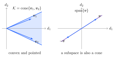
Thus a cone is invariant under nonnegative scaling. In particular, every nonempty cone contains the origin. Notice that a cone need not be convex.
A cone \mathcal K is a convex cone if, in addition,
\bm d_1,\bm d_2\in\mathcal K, \quad \alpha_1,\alpha_2\ge0 \qquad\Longrightarrow\qquad \alpha_1\bm d_1+\alpha_2\bm d_2\in\mathcal K.
Equivalently, a convex cone is closed under all nonnegative linear combinations.
Important special classes of cones are:
- a cone is pointed if \mathcal K\cap(-\mathcal K)=\{\bm0\}; geometrically, it contains no complete line through the origin;
- a cone is solid if its interior is nonempty;
- a cone is polyhedral if it can be represented as the intersection of finitely many homogeneous half-spaces, \mathcal K=\{\bm d\in\mathbb R^n:\bm A\bm d\ge\bm0\};
- a linear subspace is a special convex cone because it is closed under both positive and negative scaling.
For vectors \bm v_1,\ldots,\bm v_q\in\mathbb R^n, the cone generated by these vectors is
\operatorname{cone}\{\bm v_1,\ldots,\bm v_q\} = \left\{ \sum_{i=1}^q\alpha_i\bm v_i:\alpha_i\ge0 \right\}.
It is a finitely generated, hence polyhedral, convex cone.
A polyhedral cone from homogeneous inequalities
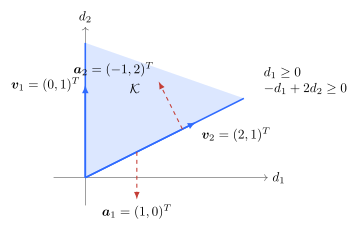
A polyhedral cone can be described either by its generating rays or by homogeneous linear inequalities. In two dimensions these two descriptions are particularly transparent. For example,
\mathcal K = \left\{\bm d\in\mathbb R^2: \begin{bmatrix} 1 & 0\\ -1 & 2 \end{bmatrix} \bm d\ge\bm0 \right\} = \operatorname{cone}\left\{ \begin{bmatrix}0\\1\end{bmatrix}, \begin{bmatrix}2\\1\end{bmatrix} \right\}.
Thus the half-space representation and the ray representation describe the same wedge. This primal/dual viewpoint is fundamental for polyhedral cones and for linearized feasible sets [5, 10].
Polar and dual cones
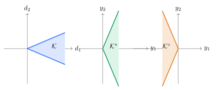
Let \mathcal K\subseteq\mathbb R^n be a cone. Its polar cone is
\mathcal K^\circ = \left\{\bm y\in\mathbb R^n: \bm y^T\bm d\le0 \quad\forall\bm d\in\mathcal K \right\},
whereas its dual cone is
\mathcal K^* = \left\{\bm y\in\mathbb R^n: \bm y^T\bm d\ge0 \quad\forall\bm d\in\mathcal K \right\}.
With these conventions,
\mathcal K^*=-\mathcal K^\circ.
Both \mathcal K^\circ and \mathcal K^* are always closed convex cones, even when \mathcal K itself is not convex. If \mathcal K is a closed convex cone, the bipolar theorem gives [5, 10]
(\mathcal K^\circ)^\circ=\mathcal K.
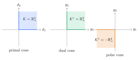
A useful two-dimensional example is the nonnegative orthant
\mathbb R_+^2=\{(d_1,d_2)^T:d_1\ge0,\ d_2\ge0\}.
It is self-dual,
(\mathbb R_+^2)^*=\mathbb R_+^2,
while its polar is the opposite orthant,
(\mathbb R_+^2)^\circ=-\mathbb R_+^2.
This simple example is worth remembering: the dual cone collects vectors having nonnegative scalar product with every vector of the original cone, whereas the polar cone uses the opposite sign.
The polar cone is particularly convenient in constrained optimization because it converts a set of admissible directions into the corresponding set of normal directions.
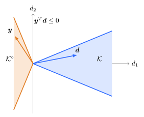
For a general wedge, the polar and dual cones need not have the same opening angle as the primal cone. If the boundary rays of \mathcal K rotate toward each other, the polar and dual cones rotate in the opposite sense and become wider. In \mathbb R^2 this angle picture is often the quickest way to understand duality.
Tangent cone and normal cone of a feasible set
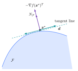
Let \mathcal F\subseteq\mathbb R^n and let \bm x^\star\in\mathcal F. The Bouligand tangent cone (also called the contingent cone) is [4, 10]
T_{\mathcal F}(\bm x^\star) = \left\{ \bm d:\; \exists\,t_j\downarrow0, \ \exists\,\bm x_j\in\mathcal F, \ \bm x_j\to\bm x^\star, \ \frac{\bm x_j-\bm x^\star}{t_j}\to\bm d \right\}.
Thus T_{\mathcal F}(\bm x^\star) contains precisely the directions that can be approached by feasible displacements at first order. If \bm x^\star is an interior point of \mathcal F, then
T_{\mathcal F}(\bm x^\star)=\mathbb R^n.
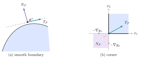
At a smooth boundary point, the tangent cone is typically a half-space; at a corner, it is typically a proper polyhedral cone.
The associated normal cone is defined as the polar of the tangent cone [4, 10],
N_{\mathcal F}(\bm x^\star) = T_{\mathcal F}(\bm x^\star)^\circ.
Consequently,
\bm y\in N_{\mathcal F}(\bm x^\star) \qquad\Longleftrightarrow\qquad \bm y^T\bm d\le0 \quad\forall\bm d\in T_{\mathcal F}(\bm x^\star).
For a differentiable objective, a local minimizer necessarily satisfies
\nabla f(\bm x^\star)\bm d\ge0 \qquad \forall\bm d\in T_{\mathcal F}(\bm x^\star),
or, equivalently,
-\nabla f(\bm x^\star)^T \in N_{\mathcal F}(\bm x^\star). \tag{4.7}
Equation Equation 4.7 is the geometric form of first-order optimality: the negative objective gradient must be a feasible-set normal.
Smooth boundary versus corner
The shape of the tangent and normal cones depends strongly on the local geometry of the feasible set. At a smooth boundary point the tangent cone is a half-space and the normal cone is a ray. At a corner the tangent cone is a proper wedge and the normal cone is itself a wedge generated by the active constraint normals. This is precisely the geometry encoded by KKT multipliers [9, 10].
Linearized cone for smooth nonlinear constraints
For the nonlinear program Equation 4.3, the first-order Taylor expansions at a feasible point \bm x^\star are
h_k(\bm x^\star+t\bm d) = t\,\nabla h_k(\bm x^\star)\bm d+o(t),
and, for every active inequality \ell\in\mathcal A(\bm x^\star),
g_\ell(\bm x^\star+t\bm d) = t\,\nabla g_\ell(\bm x^\star)\bm d+o(t).
This motivates the linearized feasible cone
\boxed{ \mathcal F_L(\bm x^\star) = \left\{ \bm d\in\mathbb R^n:\ \begin{aligned} \nabla h_k(\bm x^\star)\bm d&=0, &&k=1,\ldots,m,\\ \nabla g_\ell(\bm x^\star)\bm d&\ge0, &&\ell\in\mathcal A(\bm x^\star) \end{aligned} \right\}. } \tag{4.8}
The true tangent cone and the linearized cone satisfy, in general,
T_{\mathcal F}(\bm x^\star) \subseteq \mathcal F_L(\bm x^\star). \tag{4.9}
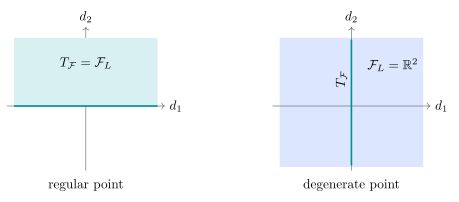
The inclusion can be strict at degenerate points. Constraint qualifications are precisely the regularity assumptions that prevent the linearized model from being too large. For example, under standard first-order regularity conditions such as MFCQ, the tangent and linearized cones coincide:
T_{\mathcal F}(\bm x^\star) = \mathcal F_L(\bm x^\star).
This equality explains geometrically why a constraint qualification is needed in order to derive KKT multipliers from first-order optimality.
The distinction between T_{\mathcal F}(\bm x^\star) and \mathcal F_L(\bm x^\star) is easiest to see in a degenerate example. Consider
\mathcal F=\{(x_1,x_2): -x_1^2\ge0\}=\{(0,x_2):x_2\in\mathbb R\}.
At the origin, the true tangent cone is the vertical line,
T_{\mathcal F}(\bm0)=\{(0,d_2):d_2\in\mathbb R\},
but \nabla g(\bm0)=\bm0, so the linearized inequality imposes no restriction and
\mathcal F_L(\bm0)=\mathbb R^2.
Thus the first-order linearization may contain many spurious directions. Constraint qualifications measure, in different strengths, how far this pathology is excluded.
With the present sign convention g_\ell\ge0, the polar of the linearized cone is generated by arbitrary combinations of equality normals and nonpositive combinations of active inequality gradients. Equivalently, its negative is generated by the active gradients with nonnegative multipliers. Therefore KKT stationarity
\nabla f(\bm x^\star) - \sum_{k=1}^m\lambda_k^\star\nabla h_k(\bm x^\star) - \sum_{\ell\in\mathcal A(\bm x^\star)} \mu_\ell^\star\nabla g_\ell(\bm x^\star) = \bm0, \qquad \mu_\ell^\star\ge0,
is exactly the multiplier representation of the geometric condition Equation 4.7.
Fritz–John conditions
Before introducing KKT conditions, it is useful to state the more general Fritz–John theorem. Its importance is conceptual: it gives first-order necessary conditions without a constraint qualification. The price is the additional multiplier \mu_0^\star, which may vanish at a degenerate solution [2, 6].
Theorem 4.1 (Fritz–John theorem) Let f, \bm h, and \bm g be continuously differentiable, and let \bm x^\star be a local minimizer of Equation 4.3. Then there exist multipliers
\mu_0^\star\ge0, \qquad \bm\lambda^\star\in\mathbb R^m, \qquad \bm\mu^\star\in\mathbb R^p, \quad \bm\mu^\star\ge\bm0,
not all zero, such that
\mu_0^\star\nabla f(\bm x^\star) -\sum_{k=1}^m\lambda_k^\star\nabla h_k(\bm x^\star) -\sum_{\ell=1}^p\mu_\ell^\star\nabla g_\ell(\bm x^\star) =\bm0,
and
\mu_\ell^\star g_\ell(\bm x^\star)=0, \qquad \ell=1,\ldots,p.
The equality multipliers \lambda_k^\star are unrestricted in sign. If \mu_0^\star>0, all multipliers may be divided by \mu_0^\star, giving the normalization \mu_0^\star=1. If \mu_0^\star=0, the point is called abnormal: stationarity is then explained entirely by the constraint gradients and contains no contribution from the objective gradient.
Constraint qualifications
A constraint qualification (CQ) is a regularity condition imposed at a feasible point. Different CQs compare the nonlinear feasible geometry with its first-order linearization at different levels of strength. Their central role is to justify the passage from geometric first-order optimality to a multiplier representation of KKT type; see, for example, [1, 2, 9].
It is useful to distinguish two mechanisms:
- LICQ and MFCQ control the active constraint gradients directly; in particular, MFCQ excludes abnormal Fritz–John multipliers;
- Abadie CQ and Guignard CQ are geometric conditions stated in terms of the tangent and linearized cones. They need not exclude degeneracy by linear independence, but they are still sufficient for first-order KKT necessity.
For smooth nonlinear programs, the standard implication chain is
\boxed{ \mathrm{LICQ} \;\Longrightarrow\; \mathrm{MFCQ} \;\Longrightarrow\; \mathrm{ACQ} \;\Longrightarrow\; \mathrm{GCQ}. } \tag{4.10}
None of the reverse implications holds in general [1, 2].
Linear independence constraint qualification (LICQ)
LICQ holds at a feasible point \bm x^\star if
\{\nabla h_k(\bm x^\star):k=1,\ldots,m\} \cup \{\nabla g_\ell(\bm x^\star):\ell\in\mathcal A(\bm x^\star)\}
is linearly independent.
LICQ is convenient and strong. Besides implying the existence of KKT multipliers at a local minimizer, it also implies uniqueness of the KKT multipliers [2, 9].
Mangasarian–Fromovitz constraint qualification (MFCQ)
Definition 4.2 MFCQ holds at a feasible point \bm x^\star if
- the equality gradients \nabla h_1(\bm x^\star),\ldots,\nabla h_m(\bm x^\star) are linearly independent; and
- there exists a direction \bm d such that
\nabla h_k(\bm x^\star)\bm d=0, \qquad k=1,\ldots,m,
and
\nabla g_\ell(\bm x^\star)\bm d>0, \qquad \ell\in\mathcal A(\bm x^\star).
For the convention g_\ell\ge0, the strict inequality points toward the interior of every active inequality.
An equivalent characterization is that
\sum_{\ell\in\mathcal A(\bm x^\star)}\alpha_\ell \nabla g_\ell(\bm x^\star) +\sum_{k=1}^m\beta_k\nabla h_k(\bm x^\star)=\bm0, \qquad \alpha_\ell\ge0,
implies \alpha_\ell=0 for every active inequality and \beta_k=0 for every equality constraint.
Thus LICQ implies MFCQ, but MFCQ permits linear dependence among the active inequality gradients. Its essential geometric content is the existence of a direction that remains tangent to all equalities while moving strictly into the interior of all active inequalities [2, 9].
Abadie constraint qualification (ACQ)
The Abadie constraint qualification is stated directly in terms of the true tangent cone and the linearized cone [1, 2].
Definition 4.3 ACQ holds at \bm x^\star if
\boxed{ T_{\mathcal F}(\bm x^\star) = \mathcal F_L(\bm x^\star). } \tag{4.11}
Since the inclusion
T_{\mathcal F}(\bm x^\star) \subseteq \mathcal F_L(\bm x^\star)
always holds for differentiable constraints, ACQ requires that every linearized feasible direction is a genuine tangent direction. In other words, the first-order linear model introduces no spurious directions.
A convenient sufficient condition for ACQ is MFCQ. Hence
\mathrm{MFCQ}\Longrightarrow\mathrm{ACQ}.
The converse is false: the tangent and linearized cones may coincide even when no single direction moves strictly into all active inequalities.
Guignard constraint qualification (GCQ)
Guignard’s condition is weaker. It does not require the tangent and linearized cones themselves to coincide; it requires only their polar cones to coincide [1, 2].
Definition 4.4 GCQ holds at \bm x^\star if
\boxed{ T_{\mathcal F}(\bm x^\star)^\circ = \mathcal F_L(\bm x^\star)^\circ. } \tag{4.12}
Because
T_{\mathcal F}(\bm x^\star) \subseteq \mathcal F_L(\bm x^\star),
polarity reverses inclusion and always gives
\mathcal F_L(\bm x^\star)^\circ \subseteq T_{\mathcal F}(\bm x^\star)^\circ.
GCQ requires only that this inclusion be an equality. Therefore ACQ immediately implies GCQ:
\mathrm{ACQ}\Longrightarrow\mathrm{GCQ}.
The importance of GCQ follows directly from the geometric first-order condition. At a local minimizer,
-\nabla f(\bm x^\star)^T \in T_{\mathcal F}(\bm x^\star)^\circ.
Under GCQ,
-\nabla f(\bm x^\star)^T \in \mathcal F_L(\bm x^\star)^\circ.
The cone \mathcal F_L(\bm x^\star) is polyhedral, so its polar has the standard multiplier representation generated by equality normals and active inequality normals. This is exactly the KKT stationarity condition. Hence GCQ is already sufficient for first-order KKT necessity.
Geometric interpretation and hierarchy of the CQs
The four qualifications can be viewed as progressively weaker requirements:
- LICQ: all active constraint normals are linearly independent;
- MFCQ: equality normals are independent and there is a strict feasible first-order direction for all active inequalities;
- ACQ: the linearized feasible cone equals the true tangent cone;
- GCQ: only the polars of these two cones must coincide.
The hierarchy is illustrated schematically below.
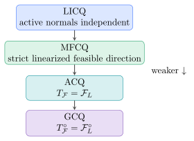
The relation between ACQ and GCQ is particularly instructive. ACQ asks for equality of feasible direction cones, whereas GCQ only asks that these cones have the same normals. Since first-order optimality depends on normals, GCQ can be sufficient for KKT even when T_{\mathcal F} and \mathcal F_L are different.
First-order feasible-arc qualification
A geometric condition stronger in spirit than merely requiring tangent-cone equality is to demand that every linearized feasible direction be realized by a feasible C^1 curve. Namely, for every \bm d satisfying
\nabla h_k(\bm x^\star)\bm d=0, \qquad \nabla g_\ell(\bm x^\star)\bm d\ge0 \quad(\ell\in\mathcal A(\bm x^\star)),
there exists a feasible C^1 curve \bm x(t) such that
\bm x(0)=\bm x^\star, \qquad \bm x'(0)=\bm d.
Such a feasible-arc property implies ACQ because every direction in the linearized cone is then, by construction, a true tangent direction.
McCormick second-order constraint qualification
McCormick’s second-order constraint qualification is a stronger geometric condition used to derive strong second-order necessary conditions. In a feasible-arc formulation, for every direction \bm d satisfying
\nabla h_k(\bm x^\star)\bm d=0, \qquad \nabla g_\ell(\bm x^\star)\bm d=0 \quad(\ell\in\mathcal A(\bm x^\star)),
one requires a twice continuously differentiable feasible curve \bm x(t), for t\ge0 sufficiently small, such that
\bm x(0)=\bm x^\star, \qquad \bm x'(0)=\bm d,
and the inequalities active at \bm x^\star remain active along the curve:
g_\ell(\bm x(t))=0, \qquad \ell\in\mathcal A(\bm x^\star).
This is a specialized second-order qualification; it should not be confused with MFCQ, which is a first-order constraint qualification [8].
KKT conditions under a constraint qualification
Under a suitable constraint qualification, the Fritz–John conditions reduce to the standard Karush–Kuhn–Tucker conditions. With the sign convention g_\ell\ge0 used in this chapter, inequality multipliers are nonnegative [3, 7, 9].
Lemma 4.1 (First-order KKT theorem) Assume that f, h_k, and g_\ell are continuously differentiable, \bm{x}^\star is a local minimizer, and a constraint qualification sufficient for KKT necessity, such as LICQ, MFCQ, ACQ, or GCQ, holds at \bm{x}^\star. Then there exist multipliers \bm{\lambda}^\star and \bm{\mu}^\star such that
\begin{aligned} \nabla_x\mathcal L(\bm{x}^\star,\bm{\lambda}^\star,\bm{\mu}^\star)&=\bm0,\\ h_k(\bm{x}^\star)&=0, && k=1,\ldots,m,\\ g_\ell(\bm{x}^\star)&\ge0, && \ell=1,\ldots,p,\\ \mu_\ell^\star&\ge0, && \ell=1,\ldots,p,\\ \mu_\ell^\star g_\ell(\bm{x}^\star)&=0, && \ell=1,\ldots,p. \end{aligned}
The last condition is complementary slackness. In particular, g_\ell(\bm{x}^\star)>0 implies \mu_\ell^\star=0.
Under LICQ the KKT multipliers are unique.
Strongly and weakly active inequalities
Once KKT multipliers are available, the active set can be split into
\begin{aligned} \mathcal A^+(\bm x^\star,\bm\mu^\star) &=\{\ell\in\mathcal A(\bm x^\star):\mu_\ell^\star>0\},\\ \mathcal A^0(\bm x^\star,\bm\mu^\star) &=\{\ell\in\mathcal A(\bm x^\star):\mu_\ell^\star=0\}. \end{aligned}
The constraints in \mathcal A^+ are called strongly active, whereas those in \mathcal A^0 are weakly active. Thus
\mathcal A^+\cap\mathcal A^0=\varnothing, \qquad \mathcal A^+\cup\mathcal A^0=\mathcal A.
This distinction is immaterial for the first-order KKT equations but becomes essential in the definition of the critical cone and in second-order optimality conditions.
From the linearized cone to the critical cone
The linearized cone contains all directions that are feasible to first order. For second-order optimality, however, only directions along which the first-order variation of the objective vanishes can be critical. This leads to the critical cone introduced next.
Critical cone
Split the active set into
\begin{aligned} \mathcal A^+(\bm{x}^\star,\bm\mu^\star) &=\{\ell\in\mathcal A(\bm{x}^\star):\mu_\ell^\star>0\},\\ \mathcal A^0(\bm{x}^\star,\bm\mu^\star) &=\{\ell\in\mathcal A(\bm{x}^\star):\mu_\ell^\star=0\}. \end{aligned}
Using the linearized feasible cone defined in Equation 4.8, the critical cone consists of those first-order feasible directions for which the first-order variation of the objective vanishes [4, 9]:
\mathcal C(\bm x^\star,\bm\mu^\star) =\{\bm d\in\mathcal F_L(\bm x^\star):\nabla f(\bm x^\star)\bm d=0\}.
At a KKT point, stationarity gives
\nabla f(\bm x^\star)\bm d = \sum_{\ell\in\mathcal A(\bm x^\star)} \mu_\ell^\star\,\nabla g_\ell(\bm x^\star)\bm d,
because the equality terms vanish for every \bm d\in\mathcal F_L. Each term on the right-hand side is nonnegative. Hence the sum can vanish only when every strongly active constraint has zero directional derivative. Thus, for the convention g_\ell\ge0,
\boxed{ \mathcal C(\bm{x}^\star,\bm\mu^\star) = \left\{\bm d:\ \begin{array}{ll} \nabla h_k(\bm{x}^\star)\bm d=0, & k=1,\ldots,m,\\ \nabla g_\ell(\bm{x}^\star)\bm d=0, & \ell\in\mathcal A^+,\\ \nabla g_\ell(\bm{x}^\star)\bm d\ge0, & \ell\in\mathcal A^0 \end{array} \right\}. } \tag{4.13}
Lemma 4.2 (Second-order necessary condition) Assume f, h_k, and g_\ell are C^2, \bm{x}^\star is a local minimizer, and LICQ holds. Let (\bm\lambda^\star,\bm\mu^\star) be the KKT multipliers. This critical-cone form is standard; see [4, 8, 9]. Then
\boxed{ \bm d^T\nabla_{xx}^2\mathcal L (\bm{x}^\star,\bm\lambda^\star,\bm\mu^\star)\bm d\ge0 \qquad \forall\bm d\in\mathcal C(\bm{x}^\star,\bm\mu^\star). }
A weaker but still valid necessary test is obtained by restricting to the smaller subspace in which all active inequalities are imposed as equalities:
\nabla g_\ell(\bm{x}^\star)\bm d=0, \qquad \ell\in\mathcal A(\bm{x}^\star).
Because this tests fewer directions, passing this weaker test does not imply that the full second-order necessary condition holds.
Lemma 4.3 (Second-order sufficient condition) Suppose that (\bm{x}^\star,\bm\lambda^\star,\bm\mu^\star) satisfies the KKT conditions. A standard sufficient condition is positivity of the Lagrangian Hessian on every nonzero critical direction [4, 9]. If
\boxed{ \bm d^T\nabla_{xx}^2\mathcal L (\bm{x}^\star,\bm\lambda^\star,\bm\mu^\star)\bm d>0 \qquad \forall\bm d\in\mathcal C(\bm{x}^\star,\bm\mu^\star)\setminus\{\bm0\}, }
then \bm{x}^\star is a strict local minimizer. Equivalently, in finite dimensions, one may require the uniform bound
\bm d^T\nabla_{xx}^2\mathcal L\,\bm d \ge \epsilon\|\bm d\|^2, \qquad \epsilon>0, \quad \bm d\in\mathcal C.
If strict complementarity holds, i.e. \mu_\ell^\star>0 for every active inequality, then \mathcal A^0=\varnothing and the critical cone reduces to the kernel of the gradients of the equality constraints and all active inequality constraints. In that special case the familiar reduced-Hessian test on that kernel is sufficient.
Without strict complementarity one must not simply replace the inequalities for weakly active constraints by equalities: doing so can miss feasible critical directions.
4.3 Notes and references
The geometric language of tangent, normal, polar, and dual cones follows the standard treatment in variational and convex analysis [4, 5, 10]. Fritz–John and KKT conditions originate in the classical works [6, 7]. For nonlinear-programming constraint qualifications and the implication relations among LICQ, MFCQ, Abadie CQ, and Guignard CQ, see [1, 2]. The critical cone and the first- and second-order optimality conditions are treated systematically in [3, 4, 9]. McCormick’s second-order condition is discussed in [8].
4.4 Chapter summary
The logical chain developed in this chapter is
\begin{array}{c} \text{feasible geometry}\\ \downarrow\\ \text{tangent/linearized cones}\\ \downarrow\\ \text{Fritz--John}\\ \downarrow\\ \text{(CQ)}\\ \downarrow\\ \text{KKT}\\ \downarrow\\ \text{critical cone}\\ \downarrow\\ \text{second-order tests} \end{array}
The key facts are:
- KKT consists of stationarity, primal feasibility, dual feasibility, and complementary slackness.
- The standard first-order CQ hierarchy is \mathrm{LICQ}\Rightarrow\mathrm{MFCQ}\Rightarrow\mathrm{ACQ}\Rightarrow\mathrm{GCQ}; GCQ is the weakest of these conditions and is already sufficient for KKT necessity.
- The second-order necessary condition requires the Lagrangian Hessian to be positive semidefinite on the critical cone.
- The corresponding sufficient condition requires strict positivity on every nonzero critical direction.
- Under strict complementarity, the critical cone becomes a linear subspace and the second-order test can be expressed through a reduced Hessian K^T H_L K.
- Weakly active constraints cannot, in general, be replaced by equalities in a second-order sufficient test.