
13 DAEs from Lagrangian Mechanics
This chapter develops nonlinear DAEs from constrained Lagrangian mechanics and discusses their numerical integration and constraint drift.
Many physical systems contain constraints that must hold throughout the motion. When such systems are formulated through the principle of stationary action, Lagrange multipliers enforce the constraints and the resulting equations are nonlinear DAEs. Unlike ODEs, these systems combine differential dynamics with algebraic geometry and require consistent initial data.
The chapter first derives constrained equations of motion from variational principles, then studies numerical integration, constraint drift, and the structural choices needed for reliable simulation and control.
13.1 Lagrangian DAEs
Foundations
This section primarily draws from the foundational works of [1] and [2]. Mechanics explores the behavior of systems ranging from particles and rigid bodies to continuous media and field theories, such as electromagnetism and gravitation. Since Newton’s formulation in the 17th century, mechanics has evolved into two dominant frameworks: Lagrangian mechanics and Hamiltonian mechanics. Here, we focus on the essentials of Lagrangian mechanics, with further details available in [2].
At the core of Lagrangian mechanics lies the principle of stationary action (or least action), a variational approach that generalizes Newton’s second law, \bm{F} = m \bm{a}. This principle provides a powerful method for deriving equations of motion for a wide range of physical systems. While both Lagrangian and Hamiltonian mechanics share this foundation, we will restrict our discussion to systems with a finite number of degrees of freedom.
Coordinates and Energies
For such systems, the configuration is described by a set of generalized coordinates:
\bm{q} := (q_{1}, q_{2}, \dots, q_{n}) \in \mathbb{R}^{n},
where n is the minimum number of independent variables needed to specify the system’s state. The choice of \bm{q} is not unique; different sets of generalized coordinates may describe the same system.
Given a coordinate system \bm{q}, we express
- the system’s kinetic energy T(\bm{q}, \dot{\bm{q}})
- and potential energy U(\bm{q}, t)
as functions of these variables. The kinetic energy depends on both positions \bm{q} and velocities \dot{\bm{q}}, while the potential energy generally depends on positions and may also explicitly depend on time t:
T: \mathbb{R}^{n} \times \mathbb{R}^{n} \to \mathbb{R}_{\geq 0}, \quad U: \mathbb{R}^{n} \times \mathbb{R} \to \mathbb{R}.
Though \bm{q} may parametrize more complex geometries (i.e., manifolds), in many practical cases, the configuration space can be locally approximated as Euclidean.
Lagrangian Function
The Lagrangian function, L(\bm{q}, \dot{\bm{q}}, t), is defined as the difference between kinetic and potential energy:
L(\bm{q}, \dot{\bm{q}}, t) := T(\bm{q}, \dot{\bm{q}}) - U(\bm{q}, t). \tag{13.1}
This function encapsulates the entire dynamics of the system and serves as the foundation for the Lagrangian formulation. Its domain consists of positions, velocities, and time:
L: \mathbb{R}^{n} \times \mathbb{R}^{n} \times \mathbb{R} \to \mathbb{R}.
Euler–Lagrange Equations
The equations of motion follow from the Euler-Lagrange equations, derived by applying the principle of stationary action:
\frac{\mathrm{d}}{\mathrm{d}t} \left( \frac{\partial L}{\partial \dot{q}_{i}} \right) - \frac{\partial L}{\partial q_{i}} = 0, \quad i = 1, \dots, n.
These equations provide a systematic method for obtaining the equations of motion for mechanical systems, from simple particles to more complex rigid-body dynamics.
The Lagrangian framework offers an elegant and unified approach to modeling physical phenomena, leveraging the principle of stationary action. By encoding dynamics in a single function L(\bm{q}, \dot{\bm{q}}, t), it simplifies problem-solving and provides deep insights into the structure of classical mechanics.
Euler–Lagrange equations
The calculus of variations used to derive the Euler–Lagrange equations is developed in Section 16.2. For a Lagrangian L(\bm{q},\dot{\bm{q}},t), stationarity of the action with fixed endpoints gives \frac{\mathrm{d}}{\mathrm{d}t} \left(\frac{\partial L}{\partial\dot{\bm{q}}}\right)^\intercal -\left(\frac{\partial L}{\partial\bm{q}}\right)^\intercal=\bm{0}. \tag{13.2}
For non-conservative generalized forces \bm{\tau}, the right-hand side becomes \bm{\tau}. The constrained form, which introduces Lagrange multipliers and algebraic equations, is developed in the section on constrained mechanics below.
Equations of Motion
While the Euler-Lagrange equations provide a general framework, it is often helpful to consider explicit representations for mechanical systems with specific characteristics. For systems where
- the kinetic energy T(\bm{q}, \dot{\bm{q}}) is a quadratic form in the generalized velocities \dot{\bm{q}},
we will derive explicit expressions for the equations of motion. This assumption is broadly applicable, as any mechanical system with a finite number of degrees of freedom can be described by a quadratic kinetic energy.
Kinetic Energy
From this foundational assumption, many interesting properties emerge. For a more comprehensive treatment, refer to [4]. The kinetic energy can be written as:
T(\bm{q}, \dot{\bm{q}}) = \frac{1}{2}\sum_{j=1}^{n}\sum_{k=1}^{n}m_{jk}(\bm{q})\dot{q}_{j}\dot{q}_{k} = \frac{1}{2}\dot{\bm{q}}^{\intercal}\bm{M}(\bm{q})\dot{\bm{q}},
where \bm{M}(\bm{q}) \in \mathbb{R}^{n \times n} is the symmetric positive definite matrix known as the mass matrix. The entries m_{jk}(\bm{q}) of \bm{M}(\bm{q}) are referred to as the generalized masses or generalized inertias.
Remark 13.1. The matrix \bm{M}(\bm{q}) is symmetric because the quadratic form associated with a matrix depends only on its symmetric part.
Derivation
We now aim to derive the explicit equations of motion for mechanical systems that exhibit quadratic kinetic energy. This process begins with the Euler-Lagrange equations, given in Equation 13.2.
First Term: Time Derivative of the Kinetic Energy
Consider the term:
\frac{\mathrm{d}}{\mathrm{d} t}\,\frac{\partial L}{\partial \dot{q}_{i}}
This term can be expressed as:
\frac{\mathrm{d}}{\mathrm{d} t}\frac{\partial L}{\partial \dot{q}_{i}} = \frac{\mathrm{d}}{\mathrm{d} t}\frac{\partial T}{\partial \dot{q}_{i}} = \frac{\mathrm{d}}{\mathrm{d} t}\frac{\partial}{\partial\dot{q}_{i}}\left(\frac{1}{2}\sum_{j=1}^{n}\sum_{k=1}^{n}m_{jk}(\bm{q})\dot{q}_{j}\dot{q}_{k}\right),
for i = 1, \ldots, n. By exploiting the linearity of summation, we can interchange the order of the partial derivative and the summation:
\begin{aligned} \frac{\mathrm{d}}{\mathrm{d} t}\frac{\partial L}{\partial \dot{q}_{i}} &= \frac{\mathrm{d}}{\mathrm{d} t}\left(\frac{1}{2}\sum_{j=1}^{n}\sum_{k=1}^{n}m_{jk}(\bm{q})\frac{\partial\dot{q}_{j}}{\partial\dot{q}_{i}}\dot{q}_{k} + \frac{1}{2}\sum_{j=1}^{n}\sum_{k=1}^{n}m_{jk}(\bm{q})\dot{q}_{j}\frac{\partial\dot{q}_{k}}{\partial\dot{q}_{i}}\right)\\ &= \frac{\mathrm{d}}{\mathrm{d} t}\left(\frac{1}{2}\sum_{k=1}^{n}m_{ik}(\bm{q})\dot{q}_{k} + \frac{1}{2}\sum_{j=1}^{n}m_{ji}(\bm{q})\dot{q}_{j}\right)\\ &= \frac{\mathrm{d}}{\mathrm{d} t}\left(\sum_{j=1}^{n}m_{ij}(\bm{q})\dot{q}_{j}\right). \end{aligned} \tag{13.3}
In the last step, we used the fact that:
\frac{\partial\dot{q}_{j}}{\partial\dot{q}_{i}} = \begin{cases} 1 & i = j \\ 0 & \text{otherwise} \end{cases}
and the symmetry condition m_{ij}(\bm{q}) = m_{ji}(\bm{q}) for i,j = 1, \ldots, n.
Taking the time derivative of this expression yields:
\frac{\mathrm{d}}{\mathrm{d} t}\frac{\partial L}{\partial\dot{q}_{i}} = \sum_{j=1}^{n}m_{ij}(\bm{q})\ddot{q}_{j} + \sum_{j=1}^{n}\sum_{k=1}^{n}\frac{\partial m_{ij}(\bm{q})}{\partial q_{k}}\dot{q}_{k}\dot{q}_{j}. \tag{13.4}
Second Term: Derivative of Potential Energy
Next, we compute the term \frac{\partial L}{\partial q_{i}}, for i=1, \ldots, n:
\frac{\partial L}{\partial q_{i}} = \frac{1}{2} \sum_{j=1}^{n}\sum_{k=1}^{n}\frac{\partial m_{jk}(\bm{q})}{\partial q_{i}}\dot{q}_{k}\dot{q}_{j} - \frac{\partial U(\bm{q}, t)}{\partial q_{i}}. \tag{13.5}
We define the following:
g_{i}(\bm{q}) := \frac{\partial U(\bm{q}, t)}{\partial q_{i}},
for i=1, \ldots, n, and the vector of generalized forces:
\bm{g}(\bm{q}) := (g_{1}(\bm{q}), \ldots, g_{n}(\bm{q})) \in \mathbb{R}^{n}.
Equations of Motion
Combining Equation 13.4 and Equation 13.5, we obtain the componentwise equations of motion:
\begin{aligned} \sum_{j=1}^{n}m_{ij}(\bm{q})\ddot{q}_{j} &+ \sum_{j=1}^{n}\sum_{k=1}^{n}\frac{\partial m_{ij}(\bm{q})}{\partial q_{k}}\dot{q}_{j}\dot{q}_{k} \\ & - \frac{1}{2}\sum_{j=1}^{n}\sum_{k=1}^{n}\frac{\partial m_{jk}(\bm{q})}{\partial q_{i}}\dot{q}_{j}\dot{q}_{k} + g_{i}(\bm{q}) = \tau_{i}, \end{aligned} \tag{13.6}
where \tau_{i} represents the generalized forces acting on the i-th degree of freedom.
Introducing Inertia Terms
To simplify, we define the following term:
h_{ijk}(\bm{q}) := \frac{\partial m_{ij}(\bm{q})}{\partial q_{k}} - \frac{1}{2}\frac{\partial m_{jk}(\bm{q})}{\partial q_{i}}. \tag{13.7}
Substituting this into Equation 13.6, we get a more compact form of the equations of motion:
\sum_{j=1}^{n}m_{ij}(\bm{q})\ddot{q}_{j} + \sum_{j=1}^{n}\sum_{k=1}^{n}h_{ijk}(\bm{q})\dot{q}_{j}\dot{q}_{k} + g_{i}(\bm{q}) = \tau_{i}, \tag{13.8}
Matrix Formulation
The equations of motion can be rewritten in compact matrix notation:
\bm{M}(\bm{q})\ddot{\bm{q}} + \bm{C}(\bm{q},\dot{\bm{q}})\dot{\bm{q}} + \bm{g}(\bm{q}) = \bm{\tau},
where \bm{C}(\bm{q},\dot{\bm{q}}) is the matrix that captures the centrifugal and Coriolis effects. The exact form of \bm{C} depends on the system’s geometry and dynamics.
Remark 13.2. It’s crucial to note that the number of degrees of freedom in a system cannot be assumed to be n - m without certain regularity conditions on the constraint function \bm{\phi}(\bm{q}, t). Specifically, if:
\text{rank}\left(\frac{\partial \bm{\phi}(\bm{q}, t)}{\partial \bm{q}}\right) = m,
then the system has exactly n - m degrees of freedom, assuming that \bm{\phi} is differentiable.
Constrained Mechanics
For mechanical systems subject to constraints, we use the method of Lagrange multipliers to handle the constraint equation
\bm{\phi}(\bm{q}, t) = 0.
The modified action \bar{S} is defined as:
\bar{S} := \int_{t_{1}}^{t_{2}} \left( L(\bm{q}, \dot{\bm{q}}, t) + \bm{\lambda}^{\intercal} \bm{\phi}(\bm{q}, t) \right) \, \mathrm{d}t,
where \bm{\lambda} \in \mathbb{R}^{m} is the vector of Lagrange multipliers. This formulation is critical for analyzing the dynamics of constrained systems.
Theorem 13.1 (Constrained Stationary Action) The motion of mechanical systems transitioning from configuration \bm{q}_{1} to \bm{q}_{2} over the time interval t \in [t_{1}, t_{2}] corresponds to the extremal curves of the functional defined in the equation above.
In other words, for small variations in the curve \bm{q}(\cdot), the modified action \bar{S} becomes stationary:
\delta \bar{S} = 0.
Remark 13.3. It is important to note that we implicitly assume that the initial and final configurations, \bm{q}_{1} and \bm{q}_{2}, satisfy the constraint equations:
\bm{\phi}(\bm{q}_{1}, t_{1}) = \bm{\phi}(\bm{q}_{2}, t_{2}) = 0.
Thus, we can perform variations as we did previously for systems with a minimal set of coordinates. However, in this case, \bar{S} also depends on the Lagrange multipliers. The variational operator \delta applies variations to \bm{q}, \dot{\bm{q}}, and \bm{\lambda}.
The result of the variation is:
\begin{aligned} \delta\bar{S} &= \int_{t_{1}}^{t_{2}} \delta L(\bm{q},\dot{\bm{q}},t) + \delta\bm{\lambda}^{\intercal}\bm{\phi}(\bm{q},t) + \bm{\lambda}^{\intercal}\delta\bm{\phi}(\bm{q},t)\, \mathrm{d}t \\ &= \int_{t_{1}}^{t_{2}}\left(\frac{\partial L}{\partial\bm{q}} - \frac{\mathrm{d}}{\mathrm{d} t}\frac{\partial L}{\partial\dot{\bm{q}}} + \bm{\lambda}^{\intercal}\frac{\partial\bm{\phi}}{\partial\bm{q}}\right)\delta\bm{q} + \delta\bm{\lambda}^{\intercal}\bm{\phi}(\bm{q},t)\, \mathrm{d}t + \left[\frac{\partial L}{\partial\dot{\bm{q}}}\delta\bm{q} \right]_{t_{1}}^{t_{2}} \\ &= \int_{t_{1}}^{t_{2}} \begin{bmatrix} \frac{\partial L}{\partial\bm{q}} - \frac{\mathrm{d}}{\mathrm{d} t}\frac{\partial L}{\partial\dot{\bm{q}}} + \bm{\lambda}^{\intercal}\frac{\partial\bm{\phi}}{\partial\bm{q}} & \bm{\phi}^{\intercal} \end{bmatrix} \begin{bmatrix} \delta\bm{q} \\ \delta\bm{\lambda} \end{bmatrix} \, \mathrm{d}t = 0. \end{aligned}
We use the fact that the variations at the endpoints are zero: \delta\bm{q}_{1} = \delta\bm{q}_{2} = 0.
Finally, applying the fundamental lemma of calculus of variations to the above expression gives:
\begin{aligned} \frac{\mathrm{d}}{\mathrm{d} t}\frac{\partial L}{\partial\dot{\bm{q}}}^{\intercal} - \frac{\partial L}{\partial \bm{q}}^{\intercal} &= \frac{\partial\bm{\phi}}{\partial\bm{q}}^{\intercal} \bm{\lambda}, \\[0.5em] \bm{\phi}(\bm{q},t) &= 0. \end{aligned}
The equations above describe the dynamics of a mechanical system subject to holonomic constraints. The term
\frac{\partial\bm{\phi}}{\partial\bm{q}}^{\intercal} \bm{\lambda}
acts as a generalized force ensuring that the constraints \bm{\phi}(\bm{q}, t) = 0 are satisfied. Unlike the equations derived from the Euler-Lagrange equations, this system involves both differential and algebraic equations, making it a Differential Algebraic Equation (DAE). Additionally, the system does not provide a direct method for determining the Lagrange multipliers.
When external non-conservative forces are present, the equations of motion modify to:
\begin{aligned} \frac{\mathrm{d}}{\mathrm{d} t}\frac{\partial L}{\partial\dot{\bm{q}}}^{\intercal} - \frac{\partial L}{\partial \bm{q}}^{\intercal} &= \frac{\partial\bm{\phi}}{\partial\bm{q}}^{\intercal} \bm{\lambda} + \bm{\tau}, \\ \bm{\phi}(\bm{q}, t) &= 0, \end{aligned}
where \bm{\tau} \in \mathbb{R}^{n} is the vector of generalized non-conservative forces.
Example 13.1 (Pendulum equations) The variational derivation of the pendulum equations, in both minimal angular coordinates and redundant Cartesian coordinates, is given in Section 16.1. Here we record the resulting equations for use in the DAE discussion.
With the minimal coordinate \theta and pendulum length l, \ddot{\theta}+\frac{g}{l}\sin\theta=0.
In redundant Cartesian coordinates \bm{q}=(x,y)^\intercal, with Lagrange multiplier \lambda, the pendulum equations are:
\begin{aligned} m\ddot{x} &= 2x\lambda,\\ m\ddot{y} &= 2y\lambda-mg,\\ x^2+y^2 &= l^2. \end{aligned}
13.2 Numerical Integration
As pointed out in [3], both from a theoretical and numerical point of view, DAEs are much more challenging than ordinary differential equations (ODEs). Some DAEs can be solved using numerical methods for stiff systems, but others cannot, and they are very sensitive to the step size, which may lead to large errors in the solution and numerical instability. For DAEs arising from constrained mechanical systems, a fairly general form is the following:
\left\{ \begin{aligned} \bm{M}(\bm{q},\bm{q}',t)\bm{q}'' - \frac{\partial\bm{\phi}(\bm{q}, t)}{\partial\bm{q}}^T \bm{\lambda} &= \bm{n}(\bm{q},\bm{q}', t), \\[0.25em] \bm{\phi}(\bm{q}, t) &= 0 \end{aligned} \right.
where the term
\bm{n}(\bm{q},\bm{q}', t) \in \mathbb{R}^{n}
collects all the contributions coming from Coriolis and centrifugal effects, conservative and non-conservative forces. It can be defined as follows:
\bm{n}(\bm{q},\bm{q}', t) = \bm{\tau} - \bm{C}(\bm{q},\bm{q}') \bm{q}' - \bm{g}(\bm{q}).
It is well known that the equations of motion for a mechanical system are a system of second-order (possibly non-linear) differential equations. However, for clarity and generality, it is useful to consider a first-order representation. For this purpose, let us define \bm{v} \in \mathbb{R}^{n} as generalized velocities, i.e.,
\bm{v} := \bm{q}'.
Thus, substituting the above equation into the general form of the equation of motion results in:
\left\{ \begin{aligned} \bm{q}' &= \bm{v}, \\[0.25em] \bm{M}(\bm{q},\bm{v},t)\bm{v}' - \frac{\partial\bm{\phi}(\bm{q}, t)}{\partial\bm{q}}^T \bm{\lambda} &= \bm{n}(\bm{q}, \bm{v}, t), \\[0.25em] \bm{\phi}(\bm{q}, t) &= 0. \end{aligned} \right. \tag{13.9}
Notice that the vector
\begin{pmatrix} \bm{q}\\ \bm{v} \end{pmatrix} \in \mathbb{R}^{2n}
represents the state of a mechanical system, namely the pair of generalized position and generalized velocity.
ODE Reduction
Now, a good question is how to solve the problem in the equation above. The issue is how to determine the value for the Lagrange multiplier \bm{\lambda}. One possible approach is to transform the problem into a system of pure differential equations. In order to do so, we need to differentiate the constraint \bm{\phi}(\bm{q}, t), which yields:
\frac{\mathrm{d}\bm{\phi}}{\mathrm{d}t} = \frac{\partial\bm{\phi}}{\partial\bm{q}} \bm{v} + \frac{\partial\bm{\phi}}{\partial t} = \bm{0}.
Notice that when the constraint does not depend on time, this expression indicates that the generalized velocity \bm{v} must be orthogonal to the gradient of the constraint. This also provides the opportunity to note that the constraint \bm{\phi}(\bm{q}, t) imposes relationships at the velocity and acceleration levels, restricting the set of feasible velocities. The constraints that we can obtain by differentiating the constraint are sometimes called hidden constraints.
Finally, notice that the equation above is still algebraic in the \bm{v} coordinate. Thus, in order to obtain a differential relationship, let us differentiate again:
\frac{\mathrm{d}^2\bm{\phi}(\bm{q}, t)}{\mathrm{d}t^2} = \frac{\mathrm{d}}{\mathrm{d}t} \left( \frac{\partial\bm{\phi}}{\partial\bm{q}} \bm{v} \right) + \frac{\partial\bm{\phi}}{\partial\bm{q}} \bm{v}' + \frac{\partial^2\bm{\phi}}{\partial t^2} = \bm{0}.
Notice that now this expression does not impose any algebraic constraint on the state of the mechanical system (\bm{q}; \bm{v}). Substituting the constraint \bm{\phi}(\bm{q}, t) = \bm{0} with the one derived above results in the following modified problem:
\left\{ \begin{aligned} \bm{q}' &= \bm{v}, \\[0.5em] \bm{M}(\bm{q},\bm{v},t)\bm{v}' - \frac{\partial\bm{\phi}(\bm{v},t)}{\partial\bm{q}}^T \bm{\lambda} &= \bm{n}(\bm{q}, \bm{v}, t), \\[0.5em] - \frac{\partial\bm{\phi}(\bm{v},t)}{\partial\bm{q}}\bm{v}' &= \bm{m}(\bm{q}, \bm{v}, t). \end{aligned} \right. \tag{13.10}
Here, to simplify the notation, we introduce the map
\bm{m}(\bm{q}, \bm{v}, t) := \frac{\mathrm{d}}{\mathrm{d}t} \left( \frac{\partial\bm{\phi}}{\partial\bm{q}} \bm{v} \right) + \frac{\partial^2\bm{\phi}}{\partial t^2}, \quad \bm{m}(\bm{q}, \bm{v}, t) \in \mathbb{R}^m.
Even though differentiating the constraint seems promising, the problem in the above equations and the one derived earlier are not equivalent. This difference leads to the so-called drift effect, which will be discussed in the next section. For now, let’s continue along the current path. The system of equations can also be written in compact matrix notation as follows:
\begin{bmatrix} \bm{I} & \bm{0} & \bm{0} \\ \bm{0} & \bm{M}(\bm{q},\bm{v},t) & -\frac{\partial\bm{\phi}}{\partial\bm{q}}^T(\bm{q},t) \\ \bm{0} & -\frac{\partial\bm{\phi}}{\partial\bm{q}}(\bm{q},t) & \bm{0} \end{bmatrix} \begin{bmatrix} \bm{q}' \\[0.5em] \bm{v}' \\[0.5em] \bm{\lambda} \end{bmatrix} = \begin{bmatrix} \bm{v} \\[0.5em] \bm{n}(\bm{q}, \bm{v}, t) \\[0.5em] \bm{m}(\bm{q}, \bm{v}, t) \end{bmatrix}.
Now, it’s easy to see that if the matrix on the left-hand side is invertible, we can express the system in explicit form and use this representation to perform numerical simulations. The matrix is invertible if and only if the sub-block:
\begin{bmatrix} \bm{M} & -\frac{\partial\bm{\phi}}{\partial\bm{q}}^T \\[0.5em] -\frac{\partial\bm{\phi}}{\partial\bm{q}} & \bm{0} \end{bmatrix} \in \mathbb{R}^{(n+m)\times(n+m)},
is non-singular (i.e., full rank).
Recall that \bm{M} is positive definite (and thus non-singular), so that
\begin{bmatrix} \bm{M} & -\frac{\partial\bm{\phi}}{\partial\bm{q}}^T \\[0.5em] -\frac{\partial\bm{\phi}}{\partial\bm{q}} & \bm{0} \end{bmatrix} = \begin{bmatrix} \bm{I} & \bm{0} \\[0.5em] -\frac{\partial\bm{\phi}}{\partial\bm{q}}\bm{M}^{-1} & \bm{I} \end{bmatrix} \begin{bmatrix} \bm{M} & \bm{0} \\[0.5em] \bm{0} & \bm{D} \end{bmatrix} \begin{bmatrix} \bm{I} & -\bm{M}^{-1}\frac{\partial\bm{\phi}}{\partial\bm{q}}^T \\[0.5em] \bm{0} & \bm{I} \end{bmatrix}
where
\bm{D} = \frac{\partial\bm{\phi}}{\partial\bm{q}} \bm{M}^{-1} \frac{\partial\bm{\phi}}{\partial\bm{q}}^T
and thus the block is non-singular if \bm{D} is non-singular.
This is not generally true, but assuming that the constraints are locally linearly independent (i.e., \forall \bm{q} \in \mathbb{R}^n, \forall t):
\text{rank}\left( \frac{\partial\bm{\phi}}{\partial\bm{q}} \right) = m,
then \bm{D} is non-singular. Thus, the system can be expressed in explicit first-order form as follows:
\begin{bmatrix} \bm{q}' \\[0.5em] \bm{v}' \\[0.5em] \bm{\lambda} \end{bmatrix} = \begin{bmatrix} \bm{I} & 0 & 0 \\ 0 & \bm{M}(\bm{q},\bm{v},t) & -\frac{\partial\bm{\phi}}{\partial\bm{q}}^T(\bm{q},t) \\ 0 & -\frac{\partial\bm{\phi}}{\partial\bm{q}}(\bm{q},t) & 0 \\ \end{bmatrix}^{-1} \begin{bmatrix} \bm{v} \\[0.5em] \bm{n}(\bm{q}, \bm{v}, t) \\[0.5em] \bm{m}(\bm{q}, \bm{v}, t) \end{bmatrix}.
An explicit expression for the inverse matrix can be obtained through tedious calculations (a calculation is done when numerical simulation are done). Regardless of the specific expression for the solution, the important point to emphasize is that by differentiating the constraint, we were able to find an explicit expression for the Lagrange multipliers. For this purpose, we differentiated twice and obtained the equation:
\bm{\lambda} = -\left( \frac{\partial\bm{\phi}}{\partial\bm{q}} \bm{M}^{-1} \frac{\partial\bm{\phi}}{\partial\bm{q}}^T \right)^{-1} \left( \frac{\mathrm{d}}{\mathrm{d}t} \frac{\partial\bm{\phi}}{\partial\bm{q}} \bm{v} + \frac{\partial\bm{\phi}}{\partial\bm{q}} \bm{M}^{-1} \bm{n}(\bm{q}, \bm{v}, t) + \frac{\partial^2\bm{\phi}}{\partial t^2} \right).
Technically, mechanical systems subject to holonomic constraints are systems of differential-algebraic equations (DAEs) of differential index 3. The differential index is one plus the number of differentiations of the constraint that are needed in order to eliminate the Lagrange multipliers. Alternatively, it is the number of times that we need to differentiate the constraint in order to obtain a differential equation for the Lagrange multiplier.
Constraint Drift
In this section we want investigate the effects of the differentiating process done to transform problem in Equation 13.9 into problem Equation 13.10. Unfortunately this method is not priceless, indeed formally we substitute an algebraic constraint with its second derivative w.r.t time. To better understand the consequences let us consider a fictitious constraint \widetilde{\bm{\phi}}(\bm{q},t) of the form,
\widetilde{\bm{\phi}}(\bm{q},t) := \bm{\phi}(\bm{q},t)+\bm{a}_0 + \bm{a}_{1}t.
It is easy to see that consider a mechanical system subject to constraint \phi(\bm{q},t) or \widetilde{\bm{\phi}}(\bm{q},t) differentiating twice is exactly the same, i.e.,
\frac{\mathrm{d}^2\bm{\phi}}{\mathrm{d} t^2} = \frac{\mathrm{d}^2\widetilde{\bm{\phi}}}{\mathrm{d} t^2}.
This fact produces the drift effect, i.e., the original constraint \bm{\phi}(\bm{q},t) is violated with an error growing with time. This error grows in the best case linearly, but it can be faster due to numerical errors. The reason of this behaviour is the term \bm{a}_{1}t which does not have any effect in the formulation Equation 13.10. Note also that this is not an undesired effect coming from not enough precision of the numerical scheme, but it is intrinsic effect due to substitution of the constraint \bm{\phi} with its second derivative w.r.t time. A simple solution to this undesired effect is the Baumgarte’s stabilization discussed in Baumgarte Stabilization.
Example 13.2 Continuing Example 13.2 we provide a first order representation for the pendulum; setting \bm{v} = \bm{q}' results,
\begin{aligned} \bm{v} &= \bm{q}',\\ m\bm{v}' + mg\bm{e}_{2} &= 2\bm{q}\lambda,\\ \bm{q}^T\bm{q} - \ell^{2} &= 0. \end{aligned}
Then in order to eliminate the Lagrange multiplier let us differentiate the constraint,
\frac{\mathrm{d}\phi}{\mathrm{d} t} = 2 \bm{q}^T\bm{v} = 0.
Notice that as expected velocity \bm{v} and position \bm{q} are orthogonal each other. Differentiating again we obtain
\frac{\mathrm{d}^{2}\phi}{\mathrm{d} t^2} = 2(\bm{q}')^T\bm{v} + 2\bm{q}^T\bm{v}' = 2\bm{v}^T\bm{v} + 2\bm{q}^T\bm{v}' = 0.
Now we can write the problem in shape of Equation 13.11,
\begin{bmatrix} \bm{I} & 0 & 0 \\[0.25em] 0 & m\bm{I} & -2\bm{q} \\[0.25em] 0 & -2\bm{q}^T & 0 \end{bmatrix} \begin{bmatrix} \bm{q}' \\[0.25em] \bm{v}' \\[0.25em] \lambda \end{bmatrix} = \begin{bmatrix} \bm{v} \\[0.25em] -mg\bm{e}_{2}\\[0.25em] 2\bm{v}^T\bm{v} \end{bmatrix}, \tag{13.11}
where \bm{I}\in\mathbb{R}^{2\times 2} is the identity matrix of dimension 2. The explicit value for the Lagrange multipliers is the following
\lambda = -\frac{m}{2\bm{q}^T\bm{q}} \left(\bm{v}^T\bm{v}-g\bm{q}^T\bm{e}_{2}\right) = -\frac{m}{2\ell^{2}}\left(\bm{v}^T\bm{v}-gq_{2}\right). \tag{13.12}
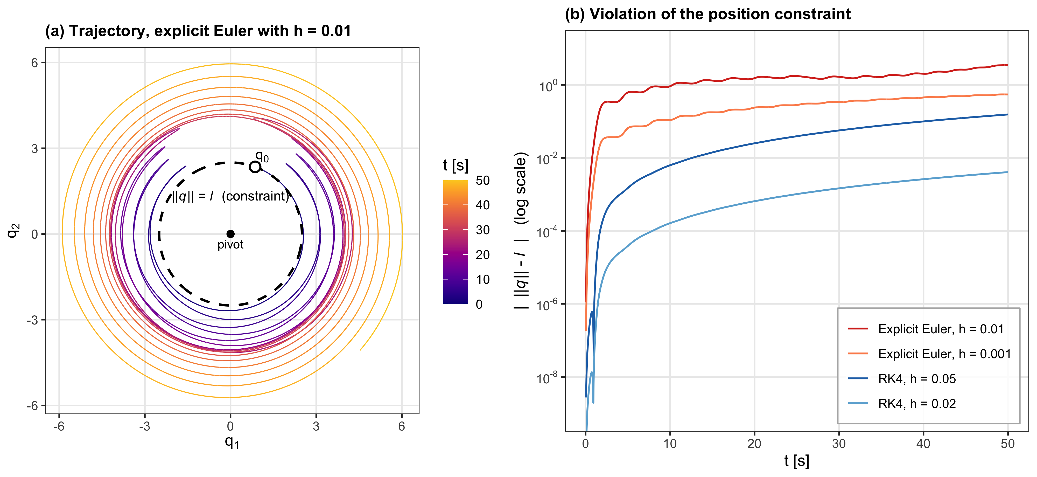
To better appreciate the drift effect we can simulate Equation 13.11 using an ODE solver: at each step \lambda is computed from Equation 13.12 and only (\bm{q},\bm{v}) are integrated. The simulation runs for 50 seconds with
- g = 9.81, m=2, \ell=2.5;
- \bm{q}_{0} \approx (0.86; 2.35)\in\mathbb{R}^{2} (projected exactly onto \|\bm{q}\|=\ell);
- \bm{q}'_{0} = \bm{v}_{0} = (0,0)\in\mathbb{R}^{2};
- \lambda_{0} = 3.69,
which are all consistent with the constraint and with Equation 13.12. The results are shown in Figure 13.1.
Both panels show that the drift is not a defect of a particular integrator. Every numerical error introduces a small perturbation of \bm{a}_0+\bm{a}_1t type, and the reduced system has no mechanism to pull the solution back onto the constraint, so the violation accumulates.