
8 Index Reduction for Linear DAEs
The Weierstrass form of Chapter 7 is valuable theoretically but expensive to compute: it requires Jordan forms, which are not numerically stable. This chapter obtains the same structural information — the separation between differential and algebraic equations, the hidden constraints, and the index — using nothing but Gaussian elimination.
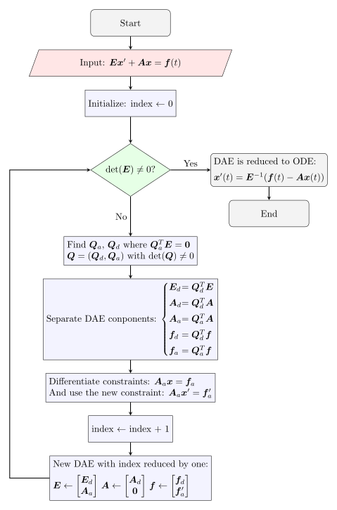
The procedure is a loop with three steps, repeated until the derivative coefficient matrix becomes nonsingular:
- separate the algebraic equations, by row-reducing \bm M=[\bm E\,|\,\bm A\,|\,\bm f] until the rows of \bm E that vanish are grouped at the bottom;
- file those algebraic equations as invariants, or hidden constraints, of the system that will result;
- differentiate them, append the result to the differential block, and start again.
Each pass through the loop reduces the index by one. What the loop produces is an ODE together with a list of invariants, and the initial condition of that ODE is not free: it must satisfy every invariant collected along the way.
8.1 Separating the Algebraic Equations
We are now prepared to explore the utility of the Gauss-like method Theorem A.1 in determining the index of a Differential-Algebraic Equation (DAE) and transforming a generic linear DAE into an Ordinary Differential Equation (ODE).
DAE Formulation
Consider a generic linear DAE expressed in the following form:
\bm{E}\bm{x}^\prime + \bm{A}\bm{x} = \bm{f}(t). \tag{8.1}
The matrices \bm{E} and \bm{A}\in \mathbb{R}^{n \times n}. Define the rank of \bm{E} as:
\text{rank}~\bm{E} = r \leq n.
Change of Coordinates
Now, consider a pair of matrices \bm{L}^{(0)} \in \mathbb{R}^{n \times n} and \bm{R}^{(0)} \in \mathbb{R}^{n \times n} such that:
\bm{L}^{(0)} \bm{E} \bm{R}^{(0)} = \bm{E}^{(0)} = \begin{bmatrix} \bm{\Lambda}^{(0)} & 0 \\ 0 & 0 \end{bmatrix}.
As in the previous section, the superscript ^{(0)} indicates the initial reduction stage; it does not by itself give the Kronecker index of the DAE. At this first iteration, \bm{\Lambda}^{(0)} \in \mathbb{R}^{r \times r}.
If r = n, we are done since the DAE has index \nu = 0, and the matrix \bm{E} is full rank and invertible. If r < n, we introduce the following change of coordinates:
\bm{x}=\bm{R}^{(0)}\bm{x}^{(0)}, \qquad \bm{x}'=\bm{R}^{(0)}(\bm{x}^{(0)})',
and define the matrix \bm{A}^{(0)} and vector \bm{f}^{(0)} as follows:
\begin{aligned} \bm{A}^{(0)} &:= \bm{L}^{(0)}\bm{A}\bm{R}^{(0)}, \\ \bm{f}^{(0)} &:= \bm{L}^{(0)}\bm{f}. \end{aligned}
so that
\bm{E}^{(0)}(\bm{x}^{(0)})' + \bm{A}^{(0)}\bm{x}^{(0)} = \bm{f}^{(0)}(t). \tag{8.2}
obtained by multiply the left-hand side of Equation 8.1 by \bm{L}^{(0)}.
Matrix Structure
Notice that by partitioning
(\bm{x}^\prime)_{1}^{(0)},\bm{x}_{1}^{(0)} \in \mathbb{R}^{r}, \quad (\bm{x}^\prime)_{2}^{(0)},\bm{x}_{2}^{(0)} \in \mathbb{R}^{n-r}, \quad \text{and} \quad \bm{x}^{(0)} = \begin{bmatrix} \bm{x}_{1}^{(0)}\\ \bm{x}_{2}^{(0)} \end{bmatrix}.
then Equation 8.2 has the following special structure:
\begin{bmatrix} \bm{\Lambda}^{(0)} & \bm{0} \\ \bm{0} & \bm{0} \end{bmatrix} \begin{bmatrix} (\bm{x}^\prime)_{1}^{(0)}(t)\\ (\bm{x}^\prime)_{2}^{(0)}(t) \end{bmatrix} + \begin{bmatrix} \bm{A}_{11}^{(0)} & \bm{A}_{12}^{(0)} \\ \bm{A}_{21}^{(0)} & \bm{A}_{22}^{(0)} \end{bmatrix} \begin{bmatrix} \bm{x}_{1}^{(0)}\\ \bm{x}_{2}^{(0)} \end{bmatrix} = \begin{bmatrix} \bm{f}_{1}^{(0)}(t)\\ \bm{f}_{2}^{(0)}(t) \end{bmatrix}. \tag{8.3}
Equation 8.3 can also be expressed as a pair of matrix equations:
\begin{aligned} \bm{\Lambda}^{(0)}(\bm{x}^\prime)_{1}^{(0)} + \bm{A}_{11}^{(0)}\bm{x}_{1}^{(0)} + \bm{A}_{12}^{(0)}\bm{x}_2^{(0)} &= \bm{f}_{1}^{(0)}(t), \qquad & (a) \\ \bm{A}_{21}^{(0)}\bm{x}_{1}^{(0)} + \bm{A}_{22}^{(0)}\bm{x}_{2}^{(0)} &= \bm{f}_{2}^{(0)}(t), \qquad & (b) \end{aligned} \tag{8.4}
Component Decoupling
Notice that
- Equation 8.4(a) is an ODE since \bm{\Lambda}^{(0)} is invertible
- Equation 8.4(b) is a pure algebraic equation.
These equations are separated by equation type, but are not generally decoupled by variable: the blocks \bm A_{12}^{(0)} and \bm A_{21}^{(0)} still couple the two groups. Actual decoupling requires further reduction (or the Weierstrass form).
Constraint Differentiation
Now we differentiate Equation 8.4(b) with respect to time:
\bm{A}_{21}^{(0)}(\bm{x}^\prime)_{1}^{(0)} + \bm{A}_{22}^{(0)}(\bm{x}^\prime)_{2}^{(0)} = (\bm{f}_2^\prime(t))^{(0)}. \tag{8.5}
Writing Equation 8.5 with Equation 8.4(a) in matrix form yields:
\begin{bmatrix} \bm{\Lambda}^{(0)} & \bm{0} \\ \bm{A}_{21}^{(0)} & \bm{A}_{22}^{(0)} \end{bmatrix} \begin{bmatrix} (\bm{x}^\prime)_{1}^{(0)}\\ (\bm{x}^\prime)_{2}^{(0)} \end{bmatrix} + \begin{bmatrix} \bm{A}_{11}^{(0)} & \bm{A}_{12}^{(0)} \\ \bm{0} & \bm{0} \end{bmatrix} \begin{bmatrix} \bm{x}_{1}^{(0)}\\ \bm{x}_{2}^{(0)} \end{bmatrix} = \begin{bmatrix} \bm{v}_{1}^{(0)}\\ (\bm{f}_2^\prime(t))^{(0)} \end{bmatrix}. \tag{8.6}
Rank Increase
As observed, the differentiation with respect to time of the algebraic constraints in the matrix representation produces merely a shift to the left of the two blocks \bm{A}_{21}^{(0)} and \bm{A}_{22}^{(0)} while preserving the original structure.
The rank of the derivative coefficient matrix need not increase strictly after differentiation. For example, if \bm A_{22}^{(0)}=\bm0, the displayed derivative matrix remains rank-deficient. Further differentiation can reveal additional constraints, but the original equations must also be retained. For a regular pencil, the nilpotency degree in the Weierstrass form gives a rigorous reference definition of the index. Rank progression alone, without specifying the precise derivative array and its independent constraints, is not an index theorem.
Definition 8.1 For a regular constant-coefficient pencil, the Kronecker index is the largest size of a nilpotent Jordan block in its Weierstrass form (index zero if no nilpotent block is present). An iterative Gaussian method may recover this number only under explicitly stated regularity and rank assumptions; the dimension of a single evolving block is not, by itself, a general definition.
In this way, we are able to compute the index of a DAE systematically through a sequence of transformations, eventually leading to a formulation where the components are decoupled, thus facilitating the analysis and solution of the DAE.
8.2 The Reduction Algorithm
A Differential-Algebraic Equation (DAE) is a system of equations that consists of both differential and algebraic equations. Unlike ordinary differential equations (ODEs), DAEs may contain constraints that restrict the solution space. The (differential) index of a DAE measures how many times the system must be differentiated to convert it into an explicit ODE.
This tutorial explains how to compute the index of a linear DAE systematically, assuming constant coefficient matrices and avoiding the Kronecker canonical form.
Reduction Procedure
First recall that a linear DAE with constant coefficients is given by:
\bm{E} \bm{x}^\prime + \bm{A} \bm{x} = \bm{f}(t)
where:
- \bm{E} and \bm{A} are constant matrices,
- \bm{x}(t) is the state variable,
- \bm{f}(t) is an input function,
- \bm{x}^\prime is the time derivative of \bm{x}.
The following steps provide a rough outline of the approach, offering a general understanding of the index reduction procedure.
Step 1: Check Singularity
Compute \det(\bm{E}):
If \det(\bm{E}) \neq 0, then \bm{E} is invertible, and the system reduces to an ODE (index 0). Terminate procedure.
If \det(\bm{E}) = 0, then \bm{E} is singular, indicating the presence of algebraic constraints. Proceed to the next step.
Step 2: Decompose the System
Determine the rank of \bm{E}\in\mathbb{R}^{n\times n}, denoted as r = \operatorname{rank}(\bm{E}). Find:
A basis \bm{Q}_a\in\mathbb{R}^{n\times (n-k)} for the null space \mathcal{N}(\bm{E}^T), which identifies the algebraic constraints.
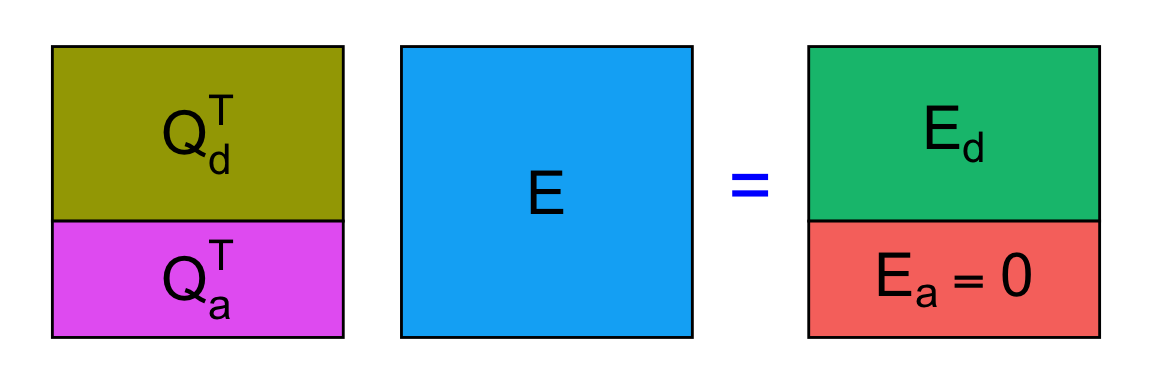
The basis satisfy \bm{E}^T\bm{Q}_a=\bm{0} or transposing \bm{Q}_a^T\bm{E}=\bm{0}.A matrix \bm{Q}_d\in\mathbb{R}^{n\times k} that complete \bm{Q}_a to a basis. In practice \bm{Q}_d make the matrix \bm{Q}=(\bm{Q}_d,\bm{Q}_a) non singular.
Decomposing the system: \bm{E} \bm{x}^\prime + \bm{A} \bm{x} = \bm{f}(t) by multiplying to the left with \bm{Q}^T:
Differential part: \bm{E}_d \bm{x}^\prime + \bm{A}_d\bm{x} = \bm{f}_d(t) where \bm{E}_d=\bm{Q}_d^T \bm{E}, \quad \bm{A}_d = \bm{Q}_d^T\bm{A}, \quad \bm{f}_d(t) = \bm{Q}_d^T\bm{f}(t)
Algebraic part: \bm{A}_a \bm{x} = \bm{f}_a(t) where \bm{A}_a = \bm{Q}_a^T\bm{A}, \qquad \bm{f}_a(t) = \bm{Q}_a^T\bm{f}(t)
since \bm{Q}_a^T \bm{E} = \bm{0}.
Remark 8.1. The decomposition used to separate differential and algebraic part seem quite cumbersome and difficult at first. However, in practice, it is straightforward to compute using standard tools from linear algebra. For instance, the LU decomposition can be applied to the matrix \bm{E} to efficiently compute \bm{Q}_A and \bm{Q}_b. The detail will be discussed forward.
Step 3: Handle Constraints
The algebraic constraints from Step 2 are:
\bm{A}_a \bm{x} = \bm{f}_a(t)).
Differentiate these constraints:
\bm{A}_a \bm{x}^\prime = \bm{f}_a^\prime (t)
Now the DAE take the form
\begin{pmatrix} \bm{E}_d \\ \bm{A}_a \end{pmatrix} \bm{x}^\prime + \begin{pmatrix} \bm{A}_d \\ \bm{0} \end{pmatrix} \bm{x} = \begin{pmatrix} \bm{f}_d(t) \\ \bm{f}_a^\prime(t) \end{pmatrix}
or
\widetilde{\bm{E}} \bm{x}^\prime + \widetilde{\bm{A}} \bm{x} = \widetilde{\bm{f}}(t)
where
\widetilde{\bm{E}}= \begin{pmatrix} \bm{E}_d \\ \bm{A}_a \end{pmatrix} \quad \widetilde{\bm{A}}= \begin{pmatrix} \bm{A}_d \\ \bm{0} \end{pmatrix} \quad \widetilde{\bm{f}}(t)= \begin{pmatrix} \bm{f}_d(t) \\ \bm{f}_a^\prime(t) \end{pmatrix}
The effect of multiply \bm{E} by \bm{Q}^T
Return to step 1. When termninate the procedure the index is the number of time Step 3 (differentiation) is performed.
Constructing the Subspaces
For the systematic construction of the matrices \bm{Q}_a and \bm{Q}_d, we leverage the (generalized) LU decomposition, which provides a structured way to separate the differential and algebraic components of a Differential-Algebraic Equation (DAE).
Let \bm{A}\in\mathbb{R}^{n \times m} of rank k\leqslant\min(n,m), then there exists two permutation matrices \bm{P}_L and \bm{P}_R such that
\bm{P}_L\bm{A}\bm{P}_R = \begin{pmatrix} \bm{L} & \bm{0} \\ \bm{M} & \bm{I} \end{pmatrix} \begin{pmatrix} \bm{U} & \bm{N} \\ \bm{0} & \bm{0} \end{pmatrix}
with
- \bm{L}\in\mathbb{R}^{k\times k} lower triangular with 1 on the main diagonal.
- \bm{U}\in\mathbb{R}^{k\times k} upper triangular with nonzero element on the main diagonal.
- \bm{M}\in\mathbb{R}^{{n-k}\times k}
- \bm{N}\in\mathbb{R}^{k\times {m-k}}
Using this theorem for \bm{E}:
\bm{P}_L\,\bm{E}\,\bm{P}_R = \begin{pmatrix} \bm{L} & \bm{0} \\ \bm{M} & \bm{I} \end{pmatrix} \begin{pmatrix} \bm{U} & \bm{N} \\ \bm{0} & \bm{0} \end{pmatrix}
and (using the fact that for a permutation matrix \bm{P}^{-1}=\bm{P}^T)
\bm{E} = \bm{P}_L^T \begin{pmatrix} \bm{L} & \bm{0} \\ \bm{M} & \bm{I} \end{pmatrix} \begin{pmatrix} \bm{U} & \bm{N} \\ \bm{0} & \bm{0} \end{pmatrix} \bm{P}_R^T
so that defining
\bm{Q}^T = \begin{pmatrix} \bm{L} & \bm{0} \\ \bm{M} & \bm{I} \end{pmatrix}^{-1} \bm{P}_L = \begin{pmatrix} \bm{L}^{-1} & \bm{0} \\ -\bm{M}\bm{L}^{-1} & \bm{I} \end{pmatrix} \bm{P}_L
we have
\begin{aligned} \bm{Q}^T\bm{E}& = \underbrace{ \begin{pmatrix} \bm{L}^{-1} & \bm{0} \\ -\bm{M}\bm{L}^{-1} & \bm{I} \end{pmatrix} \bm{P}_L }_{\bm{Q}^T} \;\; \underbrace{ \bm{P}_L^T \begin{pmatrix} \bm{L} & \bm{0} \\ \bm{M} & \bm{I} \end{pmatrix} \begin{pmatrix} \bm{U} & \bm{N} \\ \bm{0} & \bm{0} \end{pmatrix} \bm{P}_R^T }_{\bm{E}} \\[0.5em] & = \begin{pmatrix} \bm{U} & \bm{N} \\ \bm{0} & \bm{0} \end{pmatrix} \bm{P}_R^T \end{aligned}
Simplification
we can discard the colum permutation \bm{P}_R defining
\begin{pmatrix} \bm{E}_d \\ \bm{0} \end{pmatrix} = \begin{pmatrix} \bm{U} & \bm{N} \\ \bm{0} & \bm{0} \end{pmatrix} \bm{P}_R^T
so that
\bm{E} = \bm{P}_L^T \begin{pmatrix} \bm{L} & \bm{0} \\ \bm{M} & \bm{I} \end{pmatrix} \begin{pmatrix} \bm{S} \\ \bm{0} \end{pmatrix}, \quad \bm{Q}^T \bm{E} = \begin{pmatrix} \bm{E}_d \\ \bm{0} \end{pmatrix},
and applying \bm{Q}^T to the DAE \bm{E} \bm{x}^\prime + \bm{A} \bm{x} = \bm{f}(t) results in
\begin{aligned} \bm{Q}^T\left( \bm{E}\,\bm{x}^\prime+\bm{A}\,\bm{x} \right) &=\bm{Q}^T\bm{f}(t) \\[0.5em] \begin{pmatrix} \bm{E}_d \\ \bm{0} \end{pmatrix} \bm{x}^\prime +\bm{Q}^T\bm{A}\bm{x} &= \bm{Q}^T\bm{f}(t) \end{aligned}
and there is a practical separation of the algebraic equation from the DAE.
Remark 8.2 (Matrix-Free Construction). The separation of differential and algebraic part is equivalent to the reduction to echelon form (see Appendix A). This method is a systematic approach to solving linear systems, computing ranks, and checking singularity conditions.
Reduction Algorithm
Rank-based algorithms: scope and verification
A practical constant-coefficient reduction proceeds by computing a rank-revealing factorization of \bm E, applying the same row and state transformations to the entire pencil, identifying independent algebraic constraints, and differentiating them only as needed. After each step, retain the original constraints, check consistency, and recompute the ranks of the specified derivative array. Do not assume that every differentiation raises the rank. For a regular pencil, compare the inferred index against the largest nilpotent block in Weierstrass form, when that form is accessible symbolically.
8.3 Hidden Constraints as Invariants
The reduction of Section 8.2 replaces algebraic equations by their time derivatives. The resulting system is an ODE, but it is not the same problem: differentiation loses information, and what is lost must be recorded.
Consider the two-equation example
\dot x + y = 0,\qquad x = 1, \tag{8.7}
whose unique solution is x\equiv1, y\equiv0. Separating and differentiating the algebraic equation gives \dot x=0, and after one further step the explicit system
\dot x = -\tfrac12 y,\qquad \dot y = 0 . \tag{8.8}
Every solution of Equation 8.7 solves Equation 8.8, but the converse is false: Equation 8.8 admits x(t)=c_1-\tfrac12c_2t, y(t)=c_2 for every pair (c_1,c_2), a two-parameter family, whereas the DAE has exactly one solution. The ODE has more solutions than the DAE it came from.
Definition 8.2 (Invariant of an ODE) A function \bm\Psi(\bm x,t) is an invariant, or hidden constraint, of the ODE \dot{\bm x}=\bm F(\bm x,t) if
\frac{\mathrm d}{\mathrm dt}\bm\Psi(\bm x(t),t) =\frac{\partial\bm\Psi}{\partial\bm x}\bm F(\bm x,t) +\frac{\partial\bm\Psi}{\partial t} \equiv\bm0
along every solution. Its value is therefore fixed by the initial condition.
The algebraic equations discarded during index reduction are exactly the invariants of the reduced ODE. In Equation 8.7 they are x-1=0 and y=0, and the extra solutions disappear once the initial condition is required to satisfy them. This is the operational rule:
Index reduction never discards the algebraic equations: it files them as invariants of the resulting ODE, and the initial condition must satisfy them.
In the worked reductions of Section 8.4 the invariants determine the initial condition almost completely: in the three-variable example only one component of \bm x(0) remains free, the other two being forced by the hidden constraints.
Invariants of a genuine ODE
Invariants are not a DAE phenomenon. Take
\dot x = y,\qquad \dot y = -x, \qquad x(0)=1,\ y(0)=0 . \tag{8.9}
Multiplying the first equation by x, the second by y and adding gives
x\dot x+y\dot y=xy-xy=0 \quad\Longleftrightarrow\quad \frac12\frac{\mathrm d}{\mathrm dt}\bigl(x^2+y^2\bigr)=0 ,
so x^2+y^2=c is an invariant, with c=x(0)^2+y(0)^2=1 fixed by the initial data. The exact trajectory is the unit circle.
Invariants are destroyed by the integrator
A numerical method applied to Equation 8.9 does not in general preserve x^2+y^2. Explicit Euler gives
x_{k+1}=x_k+\Delta t\,y_k, \qquad y_{k+1}=y_k-\Delta t\,x_k .
Multiplying the first by x_k, the second by y_k and adding,
x_kx_{k+1}+y_ky_{k+1} =x_k^2+\Delta t\,x_ky_k+y_k^2-\Delta t\,x_ky_k =x_k^2+y_k^2 ,
that is \bm v_k\cdot\bm v_{k+1}=\|\bm v_k\|^2 with \bm v_k=(x_k,y_k)^T. By the Cauchy–Schwarz inequality |\bm v_k\cdot\bm v_{k+1}|\le\|\bm v_k\|\,\|\bm v_{k+1}\|, hence
\|\bm v_k\|^2\le\|\bm v_k\|\,\|\bm v_{k+1}\| \qquad\Longrightarrow\qquad \boxed{\;\|\bm v_{k+1}\|\ \ge\ \|\bm v_k\|\;} \tag{8.10}
The discrete trajectory spirals outwards, monotonically, for every step size: the invariant is not merely perturbed, it is violated in a fixed direction.
Implicit Euler,
x_{k+1}=x_k+\Delta t\,y_{k+1}, \qquad y_{k+1}=y_k-\Delta t\,x_{k+1} \qquad\Longleftrightarrow\qquad \begin{bmatrix}1&-\Delta t\\ \Delta t&1\end{bmatrix} \bm v_{k+1}=\bm v_k ,
reverses the inequality. Multiplying the first equation by x_{k+1}, the second by y_{k+1} and adding,
\|\bm v_{k+1}\|^2=\bm v_k\cdot\bm v_{k+1} \le\|\bm v_k\|\,\|\bm v_{k+1}\| \qquad\Longrightarrow\qquad \boxed{\;\|\bm v_{k+1}\|\ \le\ \|\bm v_k\|\;} \tag{8.11}
so the trajectory spirals inwards. Both methods converge as \Delta t\to0 on a fixed interval, and both destroy the invariant at fixed \Delta t — one by inflation, one by deflation.
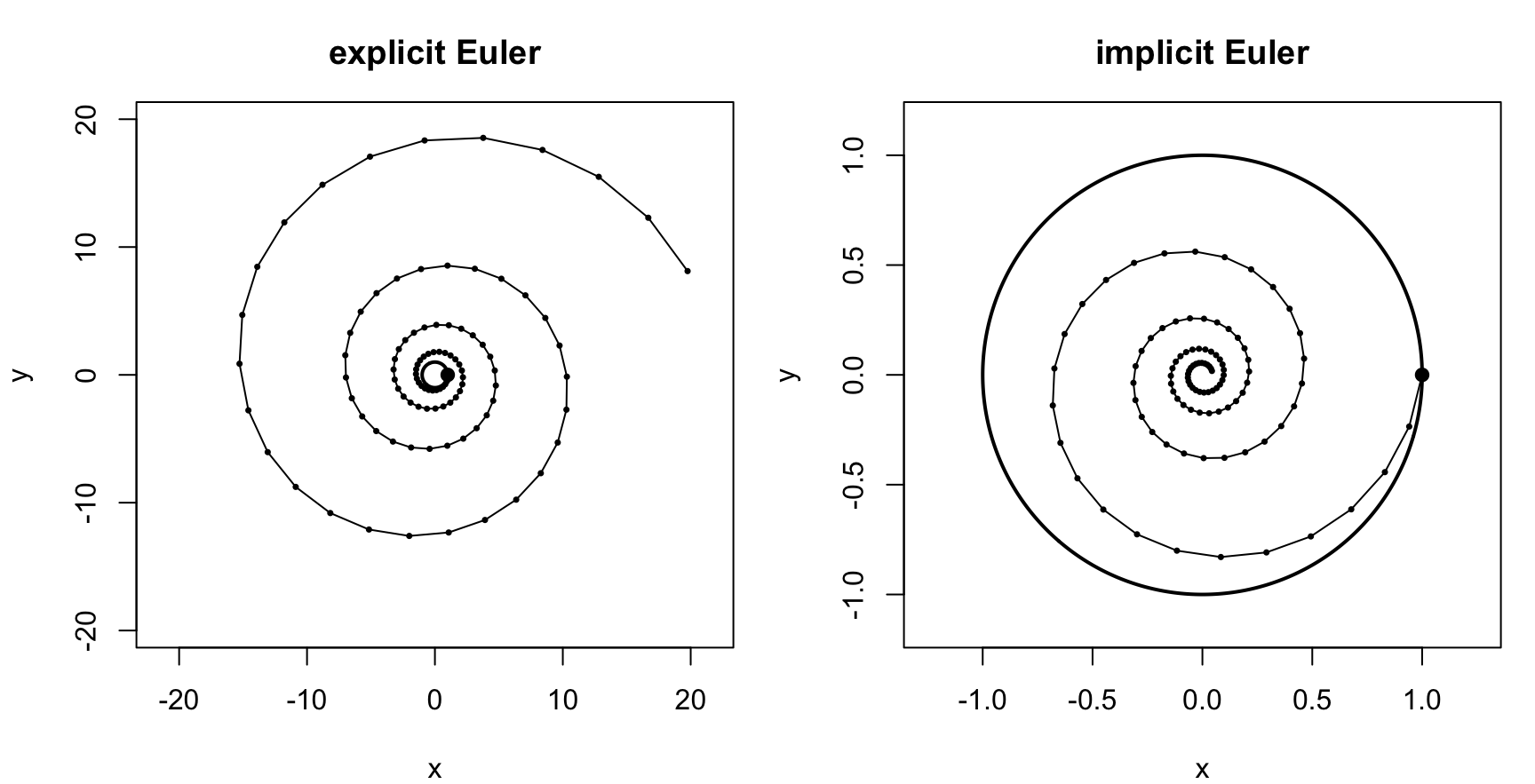
The remedy is not a smaller step but a method that respects the geometry: projection onto the constraint manifold, Baumgarte stabilization, or a structure-preserving integrator. These are the subject of Numerical Methods for DAEs, and the reason the hidden constraints produced by index reduction must be carried along with the reduced ODE rather than discarded.
8.4 Examples
The three examples below apply the algorithm of Section 8.2 in increasing order of difficulty: a system that becomes an ODE after two reductions, one that requires a row exchange, and one whose pencil is singular so that a variable can never be recovered.
Example 1: two reductions to an ODE
Linear DAE Reduction
Consider the following linear DAE:
\begin{aligned} x_1^\prime + x_2 & = 0, \\ x_1 & = 1, \end{aligned}
That written in matrix form become:
\bm{E} \bm{x}^\prime + \bm{A} \bm{x} = \bm{f}(t),
with the following matrices and vectors:
\bm{E} = \begin{bmatrix} 1 & 0 \\ 0 & 0 \end{bmatrix}, \quad \bm{A} = \begin{bmatrix} 0 & 1 \\ 1 & 0 \end{bmatrix}, \quad \bm{f}(t) = \begin{bmatrix} 0 \\ 1 \end{bmatrix}.
First reduction
Step 1: Check if \bm{E} is Singular
We compute:
\det(\bm{E}) = 0
Since \bm{E} is singular, the system is a DAE.
Step 2: Decompose the System
The basis for the null space of \bm{E}^T is: \bm{Q}_a =\begin{bmatrix}0 \\1\end{bmatrix}.
The complementary vector is: \bm{Q}_d =\begin{bmatrix} 1 \\ 0 \end{bmatrix}.
We construct the matrix \bm{Q} =\begin{bmatrix}1 & 0 \\0 & 1\end{bmatrix}.
Multiplying the system by \bm{Q}^T, we get the new matrices:
\begin{aligned} \bm{E}_d &= \bm{Q}_d^T \bm{E} &=& \begin{bmatrix} 1 & 0 \end{bmatrix} \begin{bmatrix} 1 & 0 \\ 0 & 0 \end{bmatrix} &=& \begin{bmatrix} 1 & 0 \end{bmatrix}, \\ \bm{A}_d & = \bm{Q}_d^T\bm{A} &=& \begin{bmatrix} 1 & 0 \end{bmatrix} \begin{bmatrix} 0 & 1 \\ 1 & 0 \end{bmatrix} &=& \begin{bmatrix} 0 & 1 \end{bmatrix}, \\ \bm{f}_d(t) & = \bm{Q}_d^T \bm{f}(t) &=& \begin{bmatrix} 1 & 0 \end{bmatrix} \begin{bmatrix} 0 \\ 1 \end{bmatrix} &=& \begin{bmatrix} 0 \end{bmatrix}, \\ \bm{A}_a & = \bm{Q}_a^T \bm{A} &=& \begin{bmatrix} 0 & 1 \end{bmatrix} \begin{bmatrix} 0 & 1 \\ 1 & 0 \end{bmatrix} &=& \begin{bmatrix} 1 & 0 \end{bmatrix}, \\ \bm{f}_a(t) & = \bm{Q}_a^T \bm{f}(t) &=& \begin{bmatrix} 0 & 1 \end{bmatrix} \begin{bmatrix} 0 \\ 1 \end{bmatrix} &=& \begin{bmatrix} 1 \end{bmatrix}. \end{aligned}
Step 3: Solve the System
The system becomes:
Differential part: x_1^\prime + x_2 = 0.
Algebraic part: x_1 = 1.
Differentiating the algebraic constraint x_1 = 1:
x_1^\prime = 0.
At this point the DAE become:
\widetilde{\bm{E}} \bm{x}^\prime + \widetilde{\bm{A}} \bm{x} = \widetilde{\bm{f}}(t)
with the following matrices and vectors:
\widetilde{\bm{E}} = \begin{bmatrix} 1 & 0 \\ 1 & 0 \end{bmatrix}, \quad \widetilde{\bm{A}} = \begin{bmatrix} 0 & 1 \\ 0 & 0 \end{bmatrix}, \quad \widetilde{\bm{f}}(t) = \begin{bmatrix} 0 \\ 0 \end{bmatrix}.
Second Reduction
Now reapply the algorithm:
Step 1: Check if \widetilde{\bm{E}} is Singular
We compute:
\det(\widetilde{\bm{E}}) = 0
Since \widetilde{\bm{E}} is singular, the system is still a DAE.
Step 2: Decompose the System
The basis for the null space of \widetilde{\bm{E}}^T is: \widetilde{\bm{Q}}_a =\begin{bmatrix} 1 \\ -1 \end{bmatrix}.
The complementary vector is: \widetilde{\bm{Q}}_d =\begin{bmatrix} 1 \\ 1 \end{bmatrix}.
We construct the matrix \widetilde{\bm{Q}} =\begin{bmatrix} 1 & 1 \\ 1 & -1 \end{bmatrix}.
Multiplying the system by \widetilde{\bm{Q}}^T, we get the new matrices:
\begin{aligned} \widetilde{\bm{E}}_d &= \widetilde{\bm{Q}}_d^T \widetilde{\bm{E}} &=& \begin{bmatrix} 1 & 1 \end{bmatrix} \begin{bmatrix} 1 & 0 \\ 1 & 0 \end{bmatrix} &=& \begin{bmatrix} 2 & 0 \end{bmatrix}, \\ \widetilde{\bm{A}}_d &= \widetilde{\bm{Q}}_d^T \widetilde{\bm{A}} &=& \begin{bmatrix} 1 & 1 \end{bmatrix} \begin{bmatrix} 0 & 1 \\ 0 & 0 \end{bmatrix} &=& \begin{bmatrix} 0 & 1 \end{bmatrix}, \\ \widetilde{\bm{f}}_d(t) &= \widetilde{\bm{Q}}_d^T \widetilde{\bm{f}(}t) &=& \begin{bmatrix} 1 & 1 \end{bmatrix} \begin{bmatrix} 0 \\ 0 \end{bmatrix} &=& \begin{bmatrix} 0 \end{bmatrix}, \\ \widetilde{\bm{A}}_a &= \widetilde{\bm{Q}}_a^T\widetilde{\bm{A}} &=& \begin{bmatrix} 1 & -1 \end{bmatrix} \begin{bmatrix} 0 & 1 \\ 0 & 0 \end{bmatrix} &=& \begin{bmatrix} 0 & 1 \end{bmatrix}, \\ \widetilde{\bm{f}}_a(t) &= \widetilde{\bm{Q}}_a^T \widetilde{\bm{f}}(t) &=& \begin{bmatrix} 1 & -1 \end{bmatrix} \begin{bmatrix} 0 \\ 0 \end{bmatrix} &=& \begin{bmatrix} 0 \end{bmatrix}. \end{aligned}
Step 3: Solve the System
The system becomes:
Differential part: 2x_1^\prime + x_2 = 0.
Algebraic part: x_2 = 0.
Differentiating the algebraic constraint x_2 = 0:
x_2^\prime = 0.
At this point the DAE become:
\widetilde{\widetilde{\bm{E}}} \bm{x}^\prime + \widetilde{\widetilde{\bm{A}}} \bm{x} = \widetilde{\widetilde{\bm{f}}}(t)
with the following matrices and vectors:
\widetilde{\widetilde{\bm{E}} } = \begin{bmatrix} 2 & 0 \\ 0 & 1 \end{bmatrix}, \quad \widetilde{\widetilde{\bm{A}}} = \begin{bmatrix} 0 & 1 \\ 0 & 0 \end{bmatrix}, \quad \widetilde{\widetilde{\bm{f}}}(t) = \begin{bmatrix} 0 \\ 0 \end{bmatrix}.
Now reapply the algorithm. At the step 1 \det( \widetilde{\widetilde{\bm{E}}} )=2\neq 0 so now we have an ODE:
\begin{aligned} 2x_1^\prime + x_2 &= 0, \\ x_2^\prime &= 0. \end{aligned}
we have done two derivation, thus the index of original DAE is 2.
Example 2: reduction with a row exchange
Consider the DAE
\left\{ \begin{aligned} x'(t) &= z(t)\\ z'(t) &= y(t)-t \\ x'(t) &= z(t)+x(t)+t+1 \end{aligned} \right.
define
\bm{E} = \begin{pmatrix} 1 & 0 & 0 \\ 0 & 0 & 1 \\ 1 & 0 & 0 \end{pmatrix}, \qquad \bm{A} = \begin{pmatrix} 0 & 0 & -1 \\ 0 & -1 & 0 \\ -1 & 0 & -1 \end{pmatrix}, \qquad \bm{f}(t) = \begin{pmatrix} 0 \\ -t \\ t+1 \end{pmatrix}
so that the DAE can be written as
\bm{E}\,\bm{x}^\prime(t) + \bm{A}\,\bm{x}(t) = \bm{f}(t)
The table
\bm{T} = \left[\begin{array}{c|c|c} \bm{E} & \bm{A} & \bm{f}(t) \end{array} \right] = \left[ \begin{array}{rrr|rrr|c} 1 & 0 & 0 & 0 & 0 & -1 & 0 \\ 0 & 0 & 1 & 0 & -1 & 0 & -t \\ 1 & 0 & 0 & -1 & 0 & -1 & t+1 \end{array} \right]
is used to memorize the operation done on the DAE. Let \text{index}\leftarrow 0.
Multiply table \bm{T} on the left by \bm{L}_1 where
\bm{L}_1 = \begin{pmatrix} 1 & 0 & 0 \\ 0 & 1 & 0 \\ -1 & 0 & 1 \end{pmatrix}
so that
\bm{T}_1 = \bm{L}_1\bm{T} = \left[ \begin{array}{rrr|rrr|c} 1 & 0 & 0 & 0 & 0 & -1 & 0 \\ 0 & 0 & 1 & 0 & -1 & 0 & -t \\ \hline \color{red}0 & \color{red}0 & \color{red}0 & \color{red}-1 & \color{red}0 & \color{red}0 & \color{red}t+1 \end{array} \right]
The last row contain the algebraic equation
\color{blue} -x(t) = t+1
First block now is in echelon form. Apply derivation of the last row (reduce index by one). Let \text{index}\leftarrow 1.
\bm{T}_2 = \left[ \begin{array}{rrr|rrr|c} 1 & 0 & 0 & 0 & 0 & -1 & 0 \\ 0 & 0 & 1 & 0 & -1 & 0 & -t \\ \hline \color{red}-1 & \color{red}0 & \color{red}0 & \color{red}0 & \color{red}0 & \color{red}0 & \color{red}1 \end{array} \right]
Multiply table \bm{T}_2 on the left by \bm{L}_2 where
\bm{L}_2 = \begin{pmatrix} 1 & 0 & 0 \\ 0 & 1 & 0 \\ 1 & 0 & 1 \end{pmatrix}
so that
\bm{T}_3 = \bm{L}_2\bm{T}_2 = \left[ \begin{array}{rrr|rrr|c} 1 & 0 & 0 & 0 & 0 & -1 & 0 \\ 0 & 0 & 1 & 0 & -1 & 0 & -t \\ \hline \color{red} 0 & \color{red}0 & \color{red}0 & \color{red}0 & \color{red}0 & \color{red}-1 & \color{red}1 \end{array} \right]
The last row contain the algebraic equation
\color{blue} -z(t) = 1
First block again is in echelon form. Apply derivation of the last row (reduce index by one). Let \text{index}\leftarrow 2.
\bm{T}_4 = \left[ \begin{array}{rrr|rrr|c} 1 & 0 & 0 & 0 & 0 & -1 & 0 \\ 0 & 0 & 1 & 0 & -1 & 0 & -t \\ \hline \color{red}0 & \color{red}0 & \color{red}-1 & \color{red} 0 & \color{red}0 & \color{red}0 & \color{red}0 \end{array} \right]
Multiply table \bm{T}_4 on the left by \bm{L}_4 where
\bm{L}_4 = \begin{pmatrix} 1 & 0 & 0 \\ 0 & 1 & 0 \\ 0 & 1 & 1 \end{pmatrix}
so that
\bm{T}_5 = \bm{L}_4\bm{T}_4 = \left[ \begin{array}{rrr|rrr|c} 1 & 0 & 0 & 0 & 0 & -1 & 0 \\ 0 & 0 & 1 & 0 & -1 & 0 & -t \\ \hline \color{red}0 & \color{red}0 & \color{red}0 & \color{red} 0 & \color{red}-1 & \color{red}0 & \color{red}-t \end{array} \right]
The last row contain the algebraic equation
\color{blue} -y(t) = -t
First block again is in echelon form. Apply derivation of the last row (reduce index by one). Let \text{index}\leftarrow 3.
\bm{T}_6 = \left[ \begin{array}{rrr|rrr|c} 1 & 0 & 0 & 0 & 0 & -1 & 0 \\ 0 & 0 & 1 & 0 & -1 & 0 & -t \\ \hline \color{red} 0 & \color{red}-1 & \color{red}0 & \color{red}0 & \color{red}0 & \color{red}0 & \color{red}-1 \end{array} \right]
Exchange last two rows and multily by -1 second row
\bm{P}_6 = \begin{pmatrix} 1 & 0 & 0 \\ 0 & 0 & -1 \\ 0 & 1 & 0 \end{pmatrix}
multilying \bm{T}_6 by \bm{P}_6:
\bm{P}_6\bm{T}_6 = \left[ \begin{array}{rrr|rrr|c} 1 & 0 & 0 & 0 & 0 & -1 & 0 \\ 0 & 1 & 0 & 0 & 0 & 0 & 1 \\ 0 & 0 & 1 & 0 & -1 & 0 & -t \end{array} \right]
The ODE after index reduction \left\{ \begin{aligned} x'(t) &= z(t)\\ y'(t) &= 1 \\ z'(t) &= y(t)-t \end{aligned} \right.
The algebraic (hidden) constraints
\begin{aligned} -x(t) & = t+1 \\ -z(t) & = 1 \\ -y(t) & = -t \end{aligned} \implies \left\{ \begin{aligned} x(t) & = -t-1 \\ z(t) & = -1 \\ y(t) & = t \end{aligned} \right.
The differential index is 3
Notice that the hiddent constaints determine the complete solution and the initial condition of the ODE (x(0),y(0),z(0))=(-1,-1,0).
Example 3: a singular pencil
Consider the DAE
\left\{ \begin{aligned} x'(t) &= z(t)\\ x'(t) &= y(t)-\sin t \\ x'(t) &= z(t)+y(t)+ \cos t \end{aligned} \right.
define
\bm{E} = \begin{pmatrix} 1 & 0 & 0 \\ 1 & 0 & 0 \\ 1 & 0 & 0 \end{pmatrix}, \qquad \bm{A} = \begin{pmatrix} 0 & 0 & -1 \\ 0 & -1 & 0 \\ 0 & -1 & -1 \end{pmatrix}, \qquad \bm{f}(t) = \begin{pmatrix} 0 \\ -\sin t \\ \cos t \end{pmatrix}
so that the DAE can be written as
\bm{E}\,\bm{x}^\prime(t) + \bm{A}\,\bm{x}(t) = \bm{f}(t)
The table
\bm{T} = \left[\begin{array}{c|c|c} \bm{E} & \bm{A} & \bm{f}(t) \end{array} \right] = \left[ \begin{array}{rrr|rrr|c} 1 & 0 & 0 & 0 & 0 & -1 & 0 \\ 1 & 0 & 0 & 0 & -1 & 0 & -\sin t \\ 1 & 0 & 0 & 0 & -1 & -1 & \cos t \end{array} \right]
is used to memorize the operation done on the DAE. Let \text{index}\leftarrow 0.
Multiply table \bm{T} on the left by \bm{L}_1 where
\bm{L}_1 = \begin{pmatrix} 1 & 0 & 0 \\ -1 & 1 & 0 \\ -1 & 0 & 1 \end{pmatrix}
so that
\bm{T}_1 = \bm{L}_1\bm{T} = \left[ \begin{array}{rrr|rrr|c} 1 & 0 & 0 & 0 & 0 & -1 & 0 \\ \hline \color{red}0 & \color{red}0 & \color{red}0 & \color{red}0 & \color{red}-1 & \color{red}+1 & \color{red}-\sin t \\ \color{red}0 & \color{red}0 & \color{red}0 & \color{red}0 & \color{red}-1 & \color{red} 0 & \color{red}\cos t \end{array} \right]
The last two rows contains the algebraic equations
\color{blue} -y(t)+z(t) = -\sin t, \qquad -y(t)=\cos(t)
First block now is in echelon form. Apply derivation of the last rows (reduce index by one). Let \text{index}\leftarrow 1.
\bm{T}_2 = \left[ \begin{array}{rrr|rrr|c} 1 & 0 & 0 & 0 & 0 & -1 & 0 \\ \hline \color{red}0 & \color{red}-1 & \color{red}+1 & \color{red}0 & \color{red}0 & \color{red}0 & \color{red}-\cos t \\ \color{red}0 & \color{red}-1& \color{red} 0 & \color{red}0 & \color{red}0 & \color{red}0 & \color{red}-\sin t \end{array} \right]
Multiply table \bm{T}_2 on the left by \bm{L}_2 where
\bm{L}_2 = \begin{pmatrix} 1 & 0 & 0 \\ 0 & 1 & 0 \\ 0 & -1 & 1 \end{pmatrix}
so that
\bm{T}_3 = \bm{L}_2\bm{T}_2 = \left[ \begin{array}{rrr|rrr|c} 1 & 0 & 0 & 0 & 0 & -1 & 0 \\ 0 & -1 & +1 & 0 & 0 & 0 & -\cos t \\ 0 & 0 & -1 & 0 & 0 & 0 & \cos t-\sin t \end{array} \right]
The ODE after index reduction
\begin{aligned} x'(t) & = z(t) \\ -y'(t)+z'(t) & = -\cos t \\ -z'(t) & = \cos t - \sin t \end{aligned} \implies \left\{ \begin{aligned} x'(t) & = z(t) \\ y'(t) & = \sin t \\ z'(t) & = \sin t - \cos t \end{aligned} \right.
The algebraic (hidden) constraints
\begin{aligned} -y(t)+z(t) &= -\sin t, \\ -y(t) &= \cos t \end{aligned} \implies \left\{ \begin{aligned} y(t) & = -\cos t \\ z(t) & = \cos t - \sin t \end{aligned} \right.
The differential index is 2
Notice that the hiddent constaints determine part of complete solution and the initial condition of the ODE (x(0),y(0),z(0))=(\text{free},-1,0). Thus, only z(0) must be set to determine the solution.
Worked reduction: a regular index-two pencil
Take
\bm E=\begin{bmatrix}0&1\\0&0\end{bmatrix},\qquad \bm A=\bm I_2,\qquad \bm f(t)=\begin{bmatrix}t\\t^2\end{bmatrix}, \qquad \bm E\dot{\bm x}+\bm A\bm x=\bm f.
Since \det(\bm A+\lambda\bm E)=1, the pencil is regular. The two scalar equations are
\dot x_2+x_1=t,\qquad x_2=t^2.
Differentiating the algebraic constraint gives \dot x_2=2t, hence x_1=-t. The solution is uniquely determined:
\bm x(t)=(-t,t^2)^T,\qquad \bm E\dot{\bm x}+\bm A\bm x-\bm f=\bm0.
The consistent initial condition is \bm x(0)=\bm0; prescribing x_1(0)=1 would make the IVP inconsistent. The nilpotent block is \bm E itself and has degree two, so the index is two.
Worked reduction: a singular pencil and a missing variable
Consider the three-dimensional example
\bm E=\begin{bmatrix}1&0&1\\2&0&0\\1&0&0\end{bmatrix},\quad \bm A=\begin{bmatrix}1&0&1\\0&0&0\\0&0&1\end{bmatrix},\quad \bm f(t)=\begin{bmatrix}t\\1\\t^2\end{bmatrix}, \quad \bm E\dot{\bm x}+\bm A\bm x=\bm f.
The middle column of both \bm E and \bm A is zero, so x_2 is absent from every equation. Moreover, the second and third equations yield
2\dot x_1=1,\qquad \dot x_1+x_3=t^2, \quad\Longrightarrow\quad \dot x_1=\frac12,\quad x_3=t^2-\frac12.
The first equation then requires
\dot x_3+x_1+x_3=t-\frac12 \quad\Longrightarrow\quad x_1=-t^2-t,
which contradicts \dot x_1=1/2. Thus this particular forcing is incompatible: no classical solution exists. Even for a compatible forcing, x_2(t) would remain arbitrary. This illustrates two separate pathologies of singular pencils: nonexistence and nonuniqueness.
Indeed
\det(\bm A-\lambda\bm E)\equiv0,
because its second column is identically zero. Differentiating constraints does not restore a missing equation. This is the key lesson of the final handwritten example: a formally obtained ODE for some variables need not determine the full state.
Exercises with solutions
Exercise 1 (regularity). Determine the regularity of \bm E=\operatorname{diag}(1,0) and \bm A=\operatorname{diag}(0,1). Solution: \det(\bm A-\lambda\bm E)=-\lambda is not identically zero, so the pencil is regular.
Exercise 2 (consistency). For \dot x_2+x_1=\sin t, x_2=t, determine the consistent initial state. Solution: x_1=\sin t-1, hence (x_1(0),x_2(0))=(-1,0).
Exercise 3 (index). Let \bm N be the 3\times3 nilpotent Jordan block. Determine the index and maximum derivative order of \bm g. Solution: \bm N^3=0 but \bm N^2\ne0, so the index is three and the highest derivative is \bm g''.
Exercise 4 (singularity). If \bm E and \bm A have a common zero column, can their pencil be regular? Solution: No: \bm A-\lambda\bm E has a zero column for every \lambda, hence its determinant vanishes identically.