
14 Variational Foundations
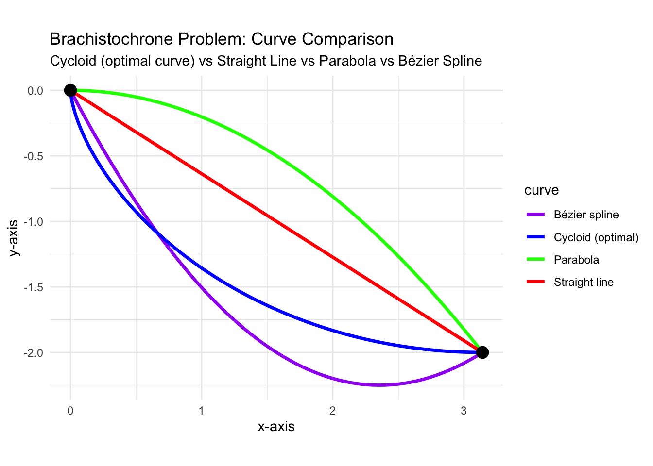
A classical problem in minimization is the brachistochrone, i.e., find the curve (meaning determining the fastest trajectory) to move from a point A to a (lower) point B considering that the only action is the one of the gravity.
example of trajectories that an object can follow for moving from point A to B.
Mathematically the problem is:
14.1 The Brachistochrone
Definition 14.1 (Problem Statement) Determine the curve
\mathcal C: [a,b] \to\mathbb{R}
such that
\mathcal C(a) = y_a \quad\text{and}\quad \mathcal C(b) = y_b
that minimize the function T(\mathcal{C}) which represent the time to travel from A=(a,y_a) to B=(b,y_b). Thus, given T(\mathcal{C}) the problem become:
\text{minimize } T(\mathcal{C}) \qquad \text{for all possible curves } \mathcal{C}
A function takes a number as input and returns a number, like f(x) = x \mathrm{e}^x. A functional is instead something that takes as input a function and returns a number and an example is
\mathcal{F}(x) = \int_a^b x(t)\,\mathrm{d}t
where x is a function. Considering for example x(t) = t^2 the previous functional becomes
\mathcal{F}(x) = \int_a^b t^2\,\mathrm{d}t = \frac{t^3}{3}\Big|_a^b= \frac{b^3-a^3}{3}
Another example of functional can be
\mathcal{G}(z) = z'(0) \int_0^1 z^2(t)\,\mathrm{d}t
and this expression can be evaluated for every generic function z(t).
The question connected to Definition 14.1 is how to define a minimum for a functional; in order to do so we have to firstly understand how to minimize a simple function and in particular given a function
f: A\subseteq\mathbb{R}\to\mathbb{R}
has a minimum in the point x^\star if
f(x^\star) \leq f(x) \qquad \forall x \in A
Similarly given a function \mathcal{F}(x) a point x^\star (that in reality is a function) is a minimum if
\mathcal{F}(x^\star) \leq \mathcal{F}(x) \qquad \forall x \in ?
In this case we have to specify the class (functional space) of functions we are considering, as example x can be a function is continuous in the domain [a,b] and so we can define
x\in C([a,b]) = \big\{ g:[a,b]\to \mathbb{R} \mid g \text{ is continuous} \big\}
In general changing the domain of the functional \mathcal{F} may change the problem.
14.2 Admissible Function Spaces
Example 14.1 (Domain-Dependence Example) For the equation f(z)=z^2+2=0, the roots exist over the complex numbers, z=\pm\mathrm{i}\sqrt{2}, but there is no solution over the real numbers.
Considering now the functional \mathcal{F} defined as
\mathcal{F}(x) = \int_{-1}^1 \big(x(t) - |t|\big)^2\, \mathrm{d}t
The |t| introduce a cuspid in t=0 that cannot be derived. If we minimize the functional in the continuous interval x\in C([-1,1]), the solution is the function x^\star(t) = |t|, in fact
\mathcal{F}(x^\star) = \int_{-1}^1 \big(|t|-|t|\big)^2 \, \mathrm{d}t = \int_{-1}^1 0\, \mathrm{d}t = 0
Choosing any other continuous function will result in a functional with a positive value.
Considering now to minimize the function in the domain of functions with continuous derivatives, and so x\in C^1([-1,1]). In this case |t|\notin C^1([-1,1]) (due to the cuspid). An approximation of the function |t| that is continuous with also continuous first derivative is the function
x_\varepsilon(t) = \begin{cases} t \qquad & t \geq \varepsilon \\ \frac 1 2 \left(\frac{t^2}\varepsilon + \varepsilon\right) \qquad & -\varepsilon < t< \varepsilon \\ -t & t \leq- \varepsilon \end{cases}
As \varepsilon\to0, this family approaches |t| and
\mathcal{F}(x_\varepsilon) = \int_{-\varepsilon}^\varepsilon \left( \frac{t^2}{2\varepsilon} + \frac \varepsilon 2 - |t| \right)^2\, \mathrm{d}t = \frac{\varepsilon^3}{10}
Therefore the infimum over C^1([-1,1]) is zero, but it is not attained: a minimizer in this space would have to coincide with |t|, which is not in C^1([-1,1]). This example distinguishes an infimum from an attained minimum.
Basic Function Spaces
- Functions f:[a,b]\mapsto\mathbb{R} continuous
- Functions f:[a,b]\mapsto\mathbb{R} which are C^k (continuous with derivative up to order k).
- Functions f:[a,b]\mapsto\mathbb{R} piecewise continuous
Lebesgue Spaces
Space L_1([a,b]) of functions f:[a,b]\mapsto\mathbb{R} which are module integrable
\int_a^b | f(t) |\,\mathrm{d}t < \infty
[the integral must exists and is finite]
Space L_2([a,b]) of functions f:[a,b]\mapsto\mathbb{R} which are square integrable
\int_a^b | f(t) |^2\,\mathrm{d}t < \infty
[the integral must exists and is finite]
Example 14.2 Let f:[0,1]\mapsto\mathbb{R}, f(x)=1/x is not L_1([0,1]) in fact
\int_0^1 \frac{1}{x}\mathrm{d}x \to \infty
The function g:[0,1]\mapsto\mathbb{R}, g(x)=1/\sqrt{x}, is in L_1([0,1]) in fact
\int_0^1 \frac{1}{\sqrt{x}}\mathrm{d}x = \left[2\sqrt{|x|}\right]_{x=0}^{x=1} =2<\infty
however this function g(x) is not in L_2([0,1]), in fact
\int_0^1 g(x)^2\mathrm{d}x= \int_0^1 \frac{1}{(\sqrt{x})^2}\mathrm{d}x= \int_0^1 \frac{1}{|x|}\mathrm{d}x \to \infty
the function h(x)=x^{-1/4} is in L_2([0,1]), in fact
\begin{aligned} \int_0^1 h(x)^2\mathrm{d}x &= \int_0^1 (x^{-1/4})^2\mathrm{d}x \\ &= \int_0^1 \frac{1}{\sqrt{x}}\mathrm{d}x\\ &= \left[2\sqrt{|x|}\right]_{x=0}^{x=1} \\ &=2<\infty \end{aligned}
14.3 Function-Space Geometry
To solve the problem of minimizing a functional we can see some relations with the linear algebra. The domain of the functional can be in fact see as a functional space \mathbb{V} analogous to the vectorial one which the vectors are represented by the functions and the scalars are represented by real values. With this definition example of functional spaces might be
\begin{aligned} \mathbb{V}_1 & = \big\{ f : [0,1] \mapsto\mathbb{R}\text{ continuous}\big\} \\ \mathbb{V}_2 & = \big\{ f: [a,b]\mapsto\mathbb{R}\text{ such that } f\in C^k([a,b]) \big\} \end{aligned}
with a,b \in \mathbb{R} and k\in \mathbb{N}.
Given in fact two function f,g \in \mathbb{V} that are member of the same functional space, we can see that each linear combination of the functions determine a function h that’s still in the vectorial space:
h(x) = \alpha f(x) + \beta g(x) \in \mathbb{V} \qquad \forall \alpha,\beta \in \mathbb{R}, \ f,g\in\mathbb{V}
As example let’s consider the two continuous function
f(x) = x^2 \quad\text{and}\quad g(x) = \sin x
then we can clearly see that the function
h(x) = 2f(x) + \frac 13 g(x) = 2x^2 +\frac 13\sin x
is still continuous. This in general means that the functional space is closed respect to the operations of function summation and multiplication by a scalar.
Inner Product
In linear algebra given two vector \bm{v}_1, \bm{v}_2 it exists the bilinear operator scalar product \langle \bm{v}_1,\bm{v}_2 \rangle = \bm{v}_1 \cdot \bm{v}_2 that satisfy the following rules:
\langle \alpha \bm{v} + \beta \bm{w}, \bm{z}\rangle = \langle \bm{z} , \alpha \bm{v} + \beta \bm{w}\rangle = \alpha \langle \bm{v},\bm{z}\rangle + \beta \langle \bm{w},\bm{z}\rangle
for all \alpha,\beta \in \mathbb{R}, \bm{v},\bm{w},\bm{z} \in \mathbb{V} and
\langle \bm{v},\bm{v}\rangle \geq 0 \quad \text{ and } \quad \langle \bm{v},\bm{v} \rangle = 0 \quad \Leftrightarrow \quad \bm{v} = \bm{0}
Also in the functional space \mathbb{V} can exists definitions of product scalar such the one here presented:
\langle f,g\rangle = \int_0^1 f(x)g(x)\, \mathrm{d}x \tag{14.1}
Note
This is one possible inner product. It is naturally defined on L^2([0,1]), whose elements are equivalence classes of functions equal almost everywhere:
\mathbb{V}=L^2([0,1]).
In this case we can prove that this definitions meets the requirements stated for the scalar product considering the linear properties of the integrals as follows:
\begin{aligned} \langle \alpha f(\cdot) + \beta g(\cdot),h \rangle & = \int_0^1 \big(\alpha f(x) + \beta g(x)\big)h(x) \, \mathrm{d}x \\ & = \alpha \int_0^1 f(x)h(x) \, \mathrm{d}x + \beta \int_0^1 g(x)h(x) \, \mathrm{d}x \\ & = \alpha \langle f,h \rangle + \beta \langle g,h \rangle \end{aligned}
and also
\langle f,f \rangle = \int_0^1 f(x)^2\,\mathrm{d}x \geq 0
Moreover, \langle f,f\rangle=0 if and only if f=0 almost everywhere.
Norm
In linear algebra it’s also defined the norm of a vector as
\|\bm{v}\| := \sqrt{\bm{v} \cdot \bm{v}}
and this expression is used to compute, from a vector, a single positive value (and in particular \|\bm{v}\| = 0 if and only if \bm{v} = \bm{0}). This definition also holds for the functional space and considering the scalar product defined (as example) in Equation 14.1 we can see that one definition of norm for function can be the one
\|f\|_{L^2} = \sqrt{\langle f,f\rangle} = \left(\int_0^1f(x)^2 \, \mathrm{d}x\right)^{1/2}
In this case we can clearly see that the norm \|f\| \geq 0 is always positive defined (and is zero only in the case on which the function f is identically null).
Example 14.3 (L^p Spaces) A space of functions can be thought of as a set of functions satisfying certain properties.
For example, one such space is the set of continuous functions f:[a,b]\to \mathbb{R}, \quad \text{with } f \in C([a,b]).
More generally, we may consider the space of k-times continuously differentiable functions f \in C^k([a,b]), \quad k \in \mathbb{N}.
Similarly, we can work with spaces of piecewise continuous functions.
A less trivial example is the space of integrable functions, namely f:[a,b]\to \mathbb{R}, \quad \text{such that } \int_a^b |f(x)|\, dx < \infty. This is precisely the space of functions that are absolutely integrable on [a,b].
In general we define as L^p([a,b]) the space of p-integrable functions, so such that
f\in L^p([a,b]) \qquad \iff \qquad \int_a^b |f(x)|^p\, \mathrm{d}x < \infty
14.4 First Variation
Let \mathcal{J}:\mathbb{V}\to\mathbb{R} be a functional defined on a function space \mathbb{V}.
To study conditions for \mathcal{J} to attain a minimum, we introduce the notion of the derivative of a functional, called the first variation (or directional derivative).
Given a function x \in \mathbb{V} and a perturbation \eta \in \mathbb{V}, we consider the variation
x_\alpha(\cdot) = x(\cdot) + \alpha \eta(\cdot), \qquad \alpha \in \mathbb{R}.
Defining the auxiliary function
g(\alpha) = \mathcal{J}\!\big(x(\cdot) + \alpha \eta(\cdot)\big).
then the first variation of \mathcal{J} at x in the direction \eta is
\delta \mathcal{J}(x;\eta) = g'(0). \tag{14.2}
Equivalent Forms
From the definition of the derivative, we can write \delta \mathcal{J}(x;\eta) = \lim_{\alpha\to 0} \frac{\mathcal{J}(x + \alpha \eta) - \mathcal{J}(x)}{\alpha}.
Equivalently, using the small-o notation, \mathcal{J}(x + \alpha \eta) = \mathcal{J}(x) + \alpha\,\delta\mathcal{J}(x;\eta) + o(\alpha).
Necessary Condition
If x^\star is an interior local minimizer and both positive and negative perturbations x^\star+\alpha\eta are admissible for sufficiently small |\alpha|, then
\delta\mathcal J(x^\star;\eta)=0 \qquad\text{for every admissible }\eta.
This is only a necessary condition: a stationary function may be a maximum or a saddle point.
Second Variation
When the second directional derivative exists, the second variation is
\delta^2\mathcal J(x;\eta) =\left.\frac{\mathrm d^2}{\mathrm d\alpha^2} \mathcal J(x+\alpha\eta)\right|_{\alpha=0}.
At a local minimizer, \delta^2\mathcal J(x^\star;\eta)\ge0 for every admissible direction. Strict positivity together with suitable coercivity gives a strict local minimum. For an integral functional
\mathcal J(x)=\int_a^b L(x,x',t)\,\mathrm dt,
the second variation along a stationary function is
\delta^2\mathcal J(x;\eta)= \int_a^b\left(L_{xx}\eta^2+2L_{x x'}\eta\eta' +L_{x'x'}(\eta')^2\right)\,\mathrm dt.
Consequently, the strengthened Legendre condition L_{x'x'}>0 is an important local convexity test. If L is jointly convex in (x,x'), every stationary admissible function is a global minimizer; strict convexity gives uniqueness.
Example 14.4 (First-Variation Example) Given the functional
\mathcal{F}(x) = \int_0^1 \big(x^2(t) + 1\big) \, \mathrm{d}t \ + x(1)
its first variation with respect to a generic direction d(t) can be calculated by first defining the scalar function g:\mathbb{R}\to\mathbb{R} as
\begin{aligned} g(\alpha) & = \mathcal{F}\big(x(\cdot) + \alpha\, d(\cdot)\big) \\ & = \int_0^1 \big(x(t) + \alpha\, d(t)\big)^2 + 1\, \mathrm{d}t + x(1) + \alpha\, d(1) \end{aligned}
As reported in Equation 14.2, the first variation of the functional \mathcal{F}(x) can be regarded as the derivative of g(\alpha) respect to \alpha evaluated for \alpha = 0; the first step is so determining
\begin{aligned} g'(\alpha ) &= \frac{\mathrm{d}}{\mathrm{d}\alpha}g(\alpha) \\ &= \frac{\mathrm{d}}{\mathrm{d}\alpha } \int_0^1 \big(x(t) + \alpha\, d(t)\big)^2 + 1\, \mathrm{d}t \\ &+ \frac{\mathrm{d}}{\mathrm{d}\alpha} \big(x(1) + \alpha\, d(1)\big) \end{aligned}
Assuming that \frac{\mathrm{d}}{\mathrm{d}\alpha}\int = \int \frac{\mathrm{d}}{\mathrm{d}\alpha} (operation that cannot always be performed) then the derivative of g(\alpha) can be regarded as
\begin{aligned} g'(\alpha) &= \int_0^1 \frac{\mathrm{d}}{\mathrm{d}\alpha} \Big(x(t) + \alpha\, d(t)\Big)^2\, \mathrm{d}t + \frac{\mathrm{d}}{\mathrm{d}\alpha} \Big(x(1) + \alpha \, d(1)\Big) \\ & = \int_0^1 2\big(x(t) + \alpha\, d(t)\big) d(t)\, \mathrm{d}t + d(1) \end{aligned}
Evaluating this expression for \alpha = 0 then the first variation of \mathcal{F}(x) with direction d(t) becomes
\delta \mathcal{F}(x;d) = g'(0) = \int_0^1 2xd\, \mathrm{d}t + d(1)
14.5 Integral Differentiation
In the computation of variations it is often assumed that \frac{\mathrm{d}}{\mathrm{d}\alpha}\circ\int_a^b \quad = \quad \int_a^b \circ \frac{\mathrm{d}}{\mathrm{d}\alpha}.
However, this property does not hold in general: some regularity conditions on the functions involved are required.
To better understand the issue, let us first examine a simpler problem.
Limit Interchange
Since a derivative is defined as a limit of a quotient, the question reduces to whether the operations of limit and integration can always be interchanged: \lim\circ\int \quad \stackrel{?}{=}\quad \int\circ\lim.
Concretely, let \{f_n\}_{n=1}^\infty be a sequence of functions such that f(x) = \lim_{n\to\infty} f_n(x), \qquad \forall x \in \mathbb{R}.
We ask whether \lim_{n\to\infty}\int_{-\infty}^{\infty} f_n(t)\,dt \stackrel{?}{=} \int_{-\infty}^{\infty}\lim_{n\to\infty} f_n(t)\,dt = \int_{-\infty}^{\infty} f(t)\,dt.
Counterexample
Consider the sequence f_n(x) = \begin{cases} 0, & x \leq 0, \\[6pt] n x, & 0 < x \leq \tfrac{1}{n}, \\[6pt] 2 - n x, & \tfrac{1}{n} < x \leq \tfrac{2}{n}, \\[6pt] 0, & x > \tfrac{2}{n}. \end{cases}
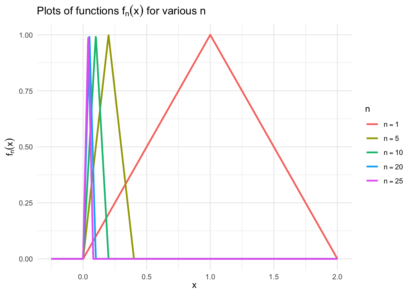
Each f_n is supported in the interval (0,2/n) and takes the shape of a triangular “bump” of base 2/n and height 1.
For every fixed x \in \mathbb{R} we have \lim_{n\to\infty} f_n(x) = 0, so the pointwise limit is the zero function: f(x) \equiv 0.
However, \int_{-\infty}^{\infty} f_n(t)\,dt = \text{area of the triangle } = \frac{1}{2}\cdot\frac{2}{n}\cdot 1 = \frac{1}{n}.
or in more detail \begin{aligned} \int_{-\infty}^\infty f_n(x)\, \mathrm{d}x &= \int_{0}^{1/n} nx \,\mathrm{d}x+ \int_{1/n}^{2/n} 2-nx \,\mathrm{d}x \\ & = \left[n\frac{x^2}{2}\right]_{x=0}^{x=1/n}+ \left[2x-n\frac{x^2}{2}\right]_{x=1/n}^{x=2/n} \\ & = \left[ n\frac{(1/n)^2}{2}-n\frac{(0)^2}{2}\right]+ \left[ 2\frac{2}{n}-n\frac{(2/n)^2}{2} -2\frac{1}{n}+n\frac{(1/n)^2}{2} \right] \\ & = \frac{1}{2n}+ \frac{4}{n}-\frac{2}{n} -\frac{2}{n}+\frac{1}{2n}=\frac{1}{n} \end{aligned}
Thus
\lim_{n\to\infty}\int_{-\infty}^{\infty} f_n(t)\,dt = 0, \qquad \int_{-\infty}^{\infty} f(t)\,dt = 0,
so in this case the interchange works.
Consider now the functions
g_n(x) = n f_n(x) = \begin{cases} 0 & x \leq 0 \\ n^2x & 0 < x \leq \frac{1}{n} \\ 2n-n^2x & \frac{1}{n} < x \leq \frac{2}{n} \\ 0 & x > \frac{2}{n} \end{cases}
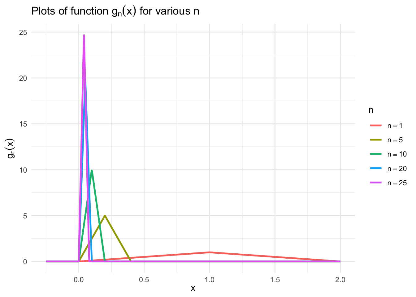
it is clear that
\lim_{n\to\infty} g_n(x) = 0,\qquad \forall x\in\mathbb{R}
and
\begin{aligned} \int_{-\infty}^\infty g_n(x)\,\mathrm{d}x &= \int_{0}^{1/n} n^2x\,\mathrm{d}x+ \int_{1/n}^{2/n} 2n-n^2x\,\mathrm{d}x \\ & = \frac{1}{2}+\frac{1}{2} = 1 \end{aligned}
and thus
\begin{aligned} \lim_{n\to\infty}\int_{-\infty}^\infty g_n(x) \mathrm{d}x & = \lim_{n\to\infty}1 = 1 \\ \int_{-\infty}^\infty \lim_{n\to\infty}g_n(x) \mathrm{d}x & = \int_{-\infty}^\infty 0 \mathrm{d}x = 0 \end{aligned}
and in this case limit and integral cannot be exchanged.
Thus limits, derivatives, and integrals cannot be interchanged without additional hypotheses.
A Sufficient Condition
A useful version of Leibniz’s rule is the following. Suppose F(t,\alpha) and \partial F/\partial\alpha are continuous on [a,b]\times(-\varepsilon,\varepsilon). Then
\frac{\mathrm d}{\mathrm d\alpha} \int_a^b F(t,\alpha)\,\mathrm dt =\int_a^b\frac{\partial F}{\partial\alpha}(t,\alpha)\,\mathrm dt.
More generally, the same conclusion follows from a dominated-convergence argument when |\partial F/\partial\alpha| is bounded by an integrable function independent of \alpha.
14.6 Local Minima and Existence
The word minimum must be qualified by the topology used on the admissible space. A function x^\star is a weak local minimizer if \mathcal F(x^\star)\leq\mathcal F(x) for all admissible x sufficiently close to x^\star in a norm controlling x and its derivatives (for example a C^1 norm). A strong local minimizer is defined using a weaker distance, typically the C^0 norm. Every global minimizer is local, but a stationary function need not be a local minimizer.
Existence is a separate question from stationarity. In modern variational analysis the direct method typically proceeds by showing:
- the admissible set is nonempty and sequentially closed in a suitable topology;
- the functional is coercive, so minimizing sequences remain bounded;
- a bounded minimizing sequence has a convergent subsequence (compactness or weak compactness);
- the functional is lower semicontinuous, so the limit attains the infimum.
For integral functionals on Sobolev spaces, convexity of the integrand with respect to the derivative variable is a standard sufficient hypothesis for weak lower semicontinuity. These hypotheses are not needed to derive Euler–Lagrange equations, but they are essential when one wants to prove that a minimizer actually exists.
14.7 Sobolev Spaces
Classical derivations often assume x\in C^1 or C^2. For existence theory the natural spaces are frequently Sobolev spaces. For example,
W^{1,p}(a,b)=\{x\in L^p(a,b):x'\in L^p(a,b)\},
where x' is the weak derivative. Boundary values are interpreted through the trace operator. This setting allows admissible minimizers whose derivatives need not be classically continuous and separates the regularity required for existence from the additional regularity needed to write the Euler–Lagrange equation pointwise.