
2 Some properties of ODEs
A system of Ordinary Differential Equations (ODEs) consists of one or more equations that describe the relationship between one or more unknown functions and their derivatives (see [1],[2])
2.1 Examples of single ODE
In this section, we present several examples of first-order ordinary differential equations, highlighting their structure and how they are defined in terms of a function f(x, y).
Example 2.1 (Nonlinear First-Order ODE**) \left\{ \begin{aligned} y' &= y^2 + x \\ y(0) &= 1 \end{aligned} \right. \implies \color{magenta} \begin{aligned} y'(x) &= y(x)^2 + x = f(x,y(x)), \\ f(x,y) &= y^2 + x \end{aligned}
Example 2.2 (ODE with Mixed Linear and Nonlinear Terms**) \left\{ \begin{aligned} y' &= xy + y^2 \\ y(0) &= 2 \end{aligned} \right. \implies \color{magenta} \begin{aligned} y'(x) &= xy(x) + y(x)^2 = f(x,y(x)), \\ f(x,y) &= xy + y^2 \end{aligned}
Example 2.3 (ODE with a Trigonometric Nonlinearity**) \left\{ \begin{aligned} z' &= x^2 + \sin z \\ z(-1) &= 0 \end{aligned} \right. \implies \color{magenta} \begin{aligned} z'(x) &= x^2 + \sin z(x) = f(x, z(x)), \\ f(x, z) &= x^2 + \sin z \end{aligned}
Example 2.4 (Logistic Growth Model (Common in Biology)**) \left\{ \begin{aligned} p' &= r p \left(1 - \frac{p}{K} \right) \\ p(0) &= p_0 \end{aligned} \right. \implies \color{magenta} p'(t) = r p(t) \left(1 - \frac{p(t)}{K} \right)
- Models population growth, where p represents the population size.
- Parameters:
- r = growth rate.
- K = carrying capacity of the environment.
- Applications: Used in ecology and epidemiology.
Example 2.5 (Newton’s Law of Cooling (Physics Application)**) \left\{ \begin{aligned} T' &= -k(T - T_{\text{env}}) \\ T(0) &= T_0 \end{aligned} \right. \implies \color{magenta} T'(t) = -k (T - T_{\text{env}})
- Describes how an object cools down over time.
- Parameters:
- k = heat transfer coefficient.
- T_{\text{env}} = ambient temperature.
2.2 Examples of Systems of ODEs
Example 2.6 (A Simple Two-Variable System) The following system describes the evolution of two state variables x(t) and y(t):
\left\{ \begin{aligned} &\left. \begin{aligned} x' & = x+y \\ y' & = \mathrm{e}^x-y \end{aligned} \right\} \quad \color{magenta} \text{ODE equations} \\ &\left. \begin{aligned} x(0) & = 1 \\ y(0) & = 1 \end{aligned} \right\} \quad \color{magenta} \text{Initial conditions} \end{aligned} \right.
- The first equation describes the rate of change of x, which depends on both x and y.
- The second equation models the evolution of y, which depends on an exponential function of x and y itself.
- The system starts from the initial state (x(0), y(0)) = (1,1).
Example 2.7 (A Three-Variable Coupled System**) This example involves three interdependent variables x, w, and z, with an explicit time dependence in the third equation.
\left\{ \begin{aligned} &\left. \begin{aligned} z' & = x+z \\ w' & = z \\ x' & = wz+t \end{aligned} \right\} \quad \color{magenta} \text{ODE equations} \\ &\left. \begin{aligned} x(0) & = 1 \\ w(0) & = 1 \\ z(0) & = 1 \\ \end{aligned} \right\} \quad \color{magenta} \text{Initial conditions} \end{aligned} \right.
2.3 Vector Form of ODEs
A system of first-order ODEs can be expressed in vector notation, which provides a more compact and structured representation of the problem. This notation is particularly useful in numerical methods and theoretical analysis.
System of ODEs in Scalar Form
Consider a system of n first-order ordinary differential equations:
y_1(t), y_2(t), \dots, y_n(t),\qquad \color{magenta} \text{functions of } t
The system is given by:
\left\{ \begin{aligned} &\left. \begin{aligned} y_1' &= f_1(t, y_1, y_2, \dots, y_n) \\ y_2' &= f_2(t, y_1, y_2, \dots, y_n) \\ &\vdots \\ y_n' &= f_n(t, y_1, y_2, \dots, y_n) \\ \end{aligned} \right\} \quad \color{magenta} \text{ODE system} \\ &\left. \begin{aligned} y_1(0) &= y_1^0, \\ y_2(0) &= y_2^0, \\ &\vdots\\ y_n(0) &= y_n^0, \end{aligned} \right\} \quad \color{magenta} \text{Initial conditions} \end{aligned} \right.
Compact Vector Form
To write this system in vector notation, define:
The state vector:
\bm{y}(t) = \begin{pmatrix} y_1(t) \\ y_2(t) \\ \vdots \\ y_n(t) \end{pmatrix}
The function that describes the system dynamics:
\bm{f}(t, \bm{y}) = \begin{pmatrix} f_1(t, y_1, y_2, \dots, y_n) \\ f_2(t, y_1, y_2, \dots, y_n) \\ \vdots \\ f_n(t, y_1, y_2, \dots, y_n) \end{pmatrix}
The initial condition vector:
\bm{y}_0 = \begin{pmatrix} y_1^0 \\ y_2^0 \\ \vdots \\ y_n^0 \end{pmatrix}
Thus, the system can be rewritten in vector form as:
\left\{ \begin{aligned} \bm{y}' &= \bm{f}(t,\bm{y}), \qquad\implies\quad \color{magenta} \bm{y}(t)=\bm{f}(t,\bm{y}(t))\\ \bm{y}(0) &= \bm{y}_0 \end{aligned} \right.
This notation simplifies analysis and computation, particularly in numerical solvers.
Matrix Form of a Linear System
When the system is linear, meaning the functions f_i(t,\bm{y}) depend linearly on \bm{y}, the system can be written as:
\bm{y}' = \bm{A}(t) \bm{y} + \bm{b}(t)
where:
- \bm{A}(t) is an n \times n matrix of coefficients.
- \bm{b}(t) is a vector of external inputs (or forcing terms).
- If \bm{b}(t) = \bm{0}, the system is homogeneous; otherwise, it is inhomogeneous.
A simple example of a homogeneous linear system is:
\begin{pmatrix} y_1' \\ y_2' \end{pmatrix} = \begin{pmatrix} a_{11} & a_{12} \\ a_{21} & a_{22} \end{pmatrix} \begin{pmatrix} y_1 \\ y_2 \end{pmatrix}
This formulation allows for powerful solution techniques, such as matrix exponentiation and eigenvalue analysis.
2.4 General ODE and properties
Before exploring numerical solution methods, it is useful to briefly review some key definitions and properties of ordinary differential equations (ODEs) and initial value problems (IVPs).
Definition 2.1 (Ordinary Differential Equation) An ordinary differential equation (ODE) is an equation involving a function z(t), defined on an interval I \subset \Bbb{R}, with values in either real or complex numbers, or in the vector spaces \Bbb{R}^d or \Bbb{C}^d. The general form of an ODE is:
\bm{f}\left(t, \bm{z}(t), \bm{z}'(t), \bm{z}''(t), \dots, \bm{z}^{(n)}(t)\right) = 0
Here, \bm{f} is a function that depends on time t, the unknown function \bm{z}(t), and its derivatives up to order n. The order of the differential equation is determined by the highest derivative \bm{z}^{(n)}(t) that appears.
If \bm{z}(t) takes values in a space of dimension d > 1, the equation is called a system of differential equations.
This form is generally too much general, the explicit form is often available in practical problems:
Definition 2.2 (Explicit ODE) An explicit first-order differential equation has the form: \bm{z}'(t) = \bm{f}\left(t, \bm{z}(t)\right) \quad \text{or briefly:} \quad \bm{z}' = \bm{f}(t, \bm{z}) \tag{2.1}
For a higher-order equation (order n), the equation is called explicit if it can be written as:
\bm{z}^{(n)}(t) = \bm{f}\left(t, \bm{z}(t), \bm{z}'(t), \bm{z}''(t), \dots, \bm{z}^{(n-1)}(t)\right)
Definition 2.3 (Autonomous ODE) A differential equation of the form Equation 2.1 is called autonomous if the right-hand side f does not explicitly depend on t, meaning:
\bm{z}'(t) = \bm{f}\left(\bm{z}(t)\right)
Numerical methods are often designed specifically for first-order ODEs. Therefore, higher-order ODEs must be transformed into an equivalent system of first-order equations before applying these methods.
Lemma 2.1 (Reduction to First-Order Systems) Every differential equation of higher order can be rewritten as a system of first-order differential equations. If the original equation is explicit, the resulting system will also be explicit.
Proof. To transform a higher-order differential equation into a system of first-order equations, we introduce auxiliary variables for each derivative of \bm{z}(t):
\begin{aligned} z_0(t) &= z(t), \\ z_1(t) &= z'(t), \\ & \vdots \\ z_{n-1}(t) & = z^{(n-1)}(t) \end{aligned}
This allows us to rewrite the original n-th order differential equation as a system of n first-order equations:
\begin{pmatrix} z'_0(t) - z_1(t) \\[0.5em] z'_1(t) - z_2(t) \\[0.5em] \vdots \\[0.5em] z'_{n-2}(t) - z_{n-1}(t) \\[0.5em] f\left(t, z_0(t), z_1(t), \dots, z_{n-1}(t), z'{n-1}(t)\right) \end{pmatrix} = \begin{pmatrix} 0 \\[0.5em] 0 \\[0.5em] \vdots \\[0.5em] 0 \\[0.5em] 0 \end{pmatrix}
In the case of an explicit equation, this system becomes:
\begin{pmatrix} z'_0(t) \\[0.5em] z'_1(t) \\[0.5em] \vdots \\[0.5em] z'_{n-2}(t) \\[0.5em] z'_{n-1}(t) \end{pmatrix} = \begin{pmatrix} z_1(t) \\[0.5em] z_2(t) \\[0.5em] \vdots \\[0.5em] z_{n-1}(t) \\[0.5em] f\left(t, z_0(t), z_1(t), \dots, z_{n-1}(t)\right) \end{pmatrix}
Most often, ODEs come with additional information in the form of an initial condition, leading to what is known as an initial value problem (IVP), also referred to as a Cauchy problem. The initial condition specifies the value of the function z at a given point t_0 within the domain, helping to define a unique solution to the differential equation.
Definition 2.4 (Initial Value Problem (IVP)) Given an initial point
(t_0,\bm{z}_0) \in \Bbb{R} \times \Bbb{R}^d
let f(t, \bm{z}(t)) be a function with values in \Bbb{R}^d, defined in a neighborhood
I \times U \subset \Bbb{R} \times \Bbb{R}^d
around the initial point. The initial value problem (IVP) is then the task of finding a function \bm{z}(t) such that:
\left\{ \begin{aligned} \bm{z}'(t) &= f(t, \bm{z}(t)) \\[0.25em] \bm{z}(t_0) &= \bm{z}_0 \end{aligned} \right.
In the study of ordinary differential equations (ODEs), the concept of a local solution plays a fundamental role in understanding the behavior of dynamical systems. Given an initial value problem (IVP), a local solution refers to a function that satisfies the differential equation and initial condition within a limited region around the initial time.
Local solutions are particularly important because existence theorems, such as the Picard-Lindelöf Theorem 2.2, often guarantee solutions only within a small interval rather than over the entire domain. This is due to factors like nonlinearities in the system, singularities, or rapidly growing solutions that may prevent global existence.
Definition 2.5 (Local Solution) A local solution to the IVP is a continuously differentiable function \bm{z}(t) that satisfies \bm{z}(t_0) = \bm{z}_0. This solution exists within some neighborhood J of t_0, where both \bm{z}(t) and \bm{f}(t, \bm{z}(t)) are well-defined, and the equation holds for all t \in J.
2.5 Well-Posedness
Definition of a Well-Posed Initial Value Problem
A mathematical problem is said to be well-posed if it satisfies the following conditions (Hadamard conditions):
- Existence: a solution exists.
- Uniqueness: the solution is unique.
- Continuous Dependence: the solution continuously depends on the initial data.
If any of these conditions fail, the problem is considered ill-posed, meaning small changes in the initial conditions can lead to large deviations in the solution.
Existence of Solutions
The following result provides a general existence theorem for first-order differential equations.
Theorem 2.1 (Peano’s Existence Theorem) Let f(t,\bm{z}) be a continuous function defined on the closed set:
\bar{D} = \left\lbrace (t, \bm{z}) \in \Bbb{R} \times \Bbb{R}^d ~\big|~ |t - t_0| \leq \alpha, |\bm{z} - \bm{z}_0| \leq \beta \right\rbrace
where \alpha, \beta > 0. Then, there exists a continuously differentiable solution \bm{z}(t) \in C^1(I) on the interval I = [t_0 - T, t_0 + T], where:
T = \min \left(\alpha, \dfrac{\beta}{M} \right), \quad M = \max_{(t, z) \in \bar{D}} |f(t, z)|
This theorem guarantees the existence of a solution but does not ensure uniqueness.
Peano’s Continuation Theorem
Under the assumptions of Peano’s Existence Theorem, the solution can be extended to a larger interval I_m = [t_-, t_+], such that the boundary points (t_-, z(t_-)) and (t_+, z(t_+)) lie on the boundary of the domain D.
- The solution exists as long as f(t, z) remains bounded.
- The interval I_m may be finite or infinite, depending on the properties of f(t, z).
2.6 Uniqueness of Solutions
To ensure uniqueness, we require stronger conditions such as Lipschitz continuity. We also introduce Grönwall’s Lemma, a crucial tool for proving uniqueness.
Lipschitz Condition
A function f(t, z) satisfies a Lipschitz condition on its domain D = I \times \Omega \subset \Bbb{R} \times \Bbb{R}^d if there exists a positive constant L such that:
\forall t \in I, \forall x, z \in \Omega : |f(t, x) - f(t, z)| \leq L |x - z|
- If L is a global constant, the function is said to satisfy a global Lipschitz condition.
- If the condition holds only for compact subsets of D, it is called a local Lipschitz condition.
The Lipschitz condition ensures uniqueness of solutions.
Grönwall’s Lemma
Grönwall’s Lemma is a fundamental result used to establish bounds on solutions and prove uniqueness.
Lemma 2.2 (Grönwall) Let
- w(t), a(t), and b(t) be non-negative, integrable functions
- the product a(t) w(t) is also integrable
- b(t) is non-decreasing
moreover w(t) satisfies the inequality:
w(t) \leq b(t) + \int_{t_0}^{t} a(s) w(s)\, \mathrm{d}s, \qquad t \geq t_0
Then for almost all t \geq t_0, we have:
w(t) \leq b(t) \exp \left( \int_{t_0}^{t} a(s)\, \mathrm{d}s \right)
This result is key in proving the uniqueness of solutions in the Picard-Lindelöf Theorem.
2.7 Existence and Uniqueness
Picard-Picard Theorem
The Picard-Lindelöf theorem (also called the Cauchy-Lipschitz theorem) strengthens Peano’s theorem by guaranteeing both existence and uniqueness of solutions.
Theorem 2.2 (Picard-Lindelöf) Let f(t,\bm{z}) be continuous on the cylinder:
D = \{ (t, \bm{z}) \in \Bbb{R} \times \Bbb{R}^d ~\big|~ |t - t_0| \leq a, |\bm{z} - \bm{z}_0| \leq b \}
Assume that:
\bm{f}(t, \bm{z}) is bounded, meaning there exists a constant M such that:
\|\bm{f}(t, \bm{z})\| \leq M, \quad \forall (t, \bm{z}) \in D
f satisfies a Lipschitz condition with constant L:
\|\bm{f}(t, \bm{x}) - \bm{f}(t, \bm{z})\| \leq L \|\bm{x} - \bm{z}\|, \quad \forall \bm{x}, \bm{z} \in D
Then, the initial value problem:
\left\{ \begin{aligned} \bm{z}'(t) &= \bm{f}(t, \bm{z}(t)) \\[0.25em] \bm{z}(t_0) &= \bm{z}_0 \end{aligned} \right.
has a unique solution on the interval I = [t_0 - T, t_0 + T], where:
T = \min \left( a, \dfrac{b}{M} \right)
2.8 Example of ODE with Existence but No Uniqueness
Consider the ordinary differential equation (ODE):
y' = \sqrt{|y|}
with the initial condition:
y(0) = 0.
Existence of the Solution
Peano’s Theorem guarantees that if a function f(t, y) is continuous, then there exists at least one solution within some interval around the initial point. In this case, the function f(y) = \sqrt{|y|} is continuous for all values of y, so Peano’s theorem tells us that there exists at least one solution for the given ODE, at least in a small interval around t = 0.
Thus, we can assert that there exists a function y(t) that satisfies the differential equation and the initial condition y(0) = 0.
No Uniqueness of the Solution
Picard-Lindelöf Theorem 2.2 states that, in addition to existence, a solution is also unique if the function f(t, y) is Lipschitz continuous with respect to y in an interval around the initial condition y_0. However, in our case, the function f(y) = \sqrt{|y|} is not Lipschitz continuous at y = 0.
To verify this, let’s compute the derivative of f(y) = \sqrt{|y|}:
f'(y) = \left\{ \begin{aligned} \frac{1}{2\sqrt{y}} & y \geq 0 \\[0.5em] -\frac{1}{2\sqrt{-y}} & y \geq 0 \end{aligned} \right. =\frac{\textrm{sign}(y)}{2\sqrt{|y|}}
Notice that this derivative becomes infinite as y \to 0, so the function is not Lipschitz continuous at y = 0. The Lipschitz condition requires the derivative to be bounded, but in this case, it is not.
Since f(y) = \sqrt{|y|} does not satisfy the Lipschitz condition at y = 0, Picard-Lindelöf Theorem 2.2 does not guarantee the uniqueness of the solution. This means there may be more than one solution that satisfies the same initial condition y(0) = 0.
Multiple Solutions
Even though a solution exists, it is not unique. In fact, there are many solutions that satisfy the ODE and the initial condition y(0) = 0. Here are a few examples:
Trivial (Zero) Solution
One solution is the zero solution, where y(x) = 0 for all x. This is a solution that satisfies both the ODE and the initial condition y(0) = 0, and it holds for every value of x.
y(x) = 0 \quad \text{for all} \quad x.
Explicit (Non-Zero) Solution
Another solution can be found by solving the ODE by separating the variables. We start by writing the ODE as:
\frac{\mathrm{d}y}{\sqrt{|y|}} = \mathrm{d}x.
Integrating both sides:
2\sqrt{|y|} = x + C.
Setting the initial condition y(0) = 0, we get C = 0. Therefore, the solution becomes:
y(x) = \frac{x^2}{4}, \quad \text{for} \quad x \geq 0.
This is an explicit solution for x \geq 0 and satisfies the ODE and the initial condition.
For x < 0, the solution must be:
y(x) = -\frac{x^2}{4}, \quad \text{for} \quad x < 0,
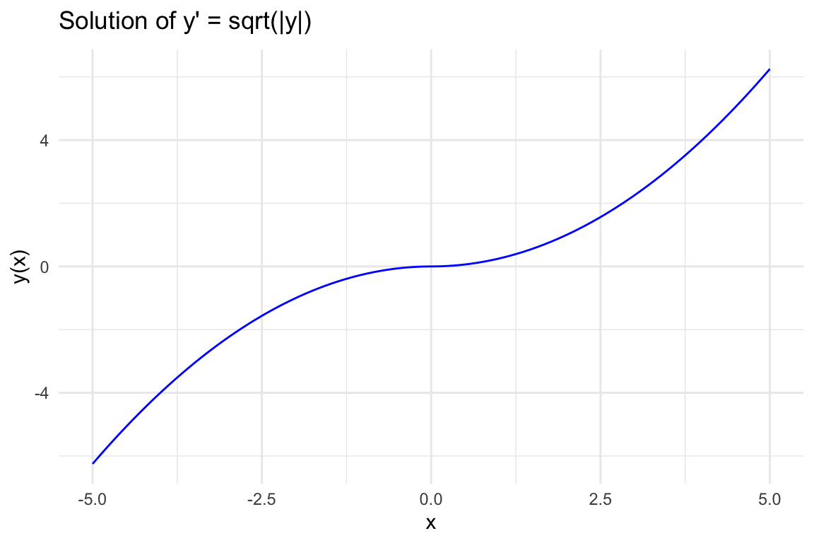
to match the sign of the right-hand side. Thus, the complete solution is:
y(x) = \dfrac{x^2}{4} \begin{cases} 1 & x \geq 0, \\ -1 & x < 0. \end{cases}
This can also be written more compactly as:
y(x) = \dfrac{x|x|}{4}.
The derivative of this function is:
y'(x) = \dfrac{x}{2} \begin{cases} 1 & x \geq 0, \\ -1 & x < 0. \end{cases}
Which simplifies to:
y'(x) = \dfrac{|x|}{2}.
Notice that:
\sqrt{|y(x)|} = \sqrt{\left|\dfrac{x|x|}{4}\right|} = \sqrt{\dfrac{|x|^2}{4}} = \dfrac{|x|}{2} = y'(x).
Thus, the function y(x) = \dfrac{x|x|}{4} satisfies the ODE, and it is indeed a valid solution.
Conclusion
The ODE y' = \sqrt{|y|} with the initial condition y(0) = 0 has multiple solutions. In addition to the trivial solution y(x) = 0, we also have non-zero solutions of the form:
y(x) = \dfrac{x|x|}{4}.
These multiple solutions are possible due to the lack of uniqueness in this case, as the function f(y) = \sqrt{|y|} is not Lipschitz continuous at y = 0.