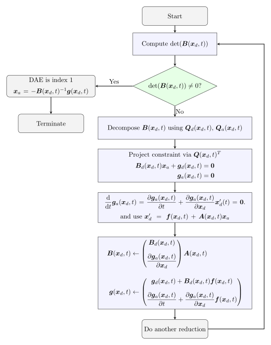
14 Index Reduction of DAEs Using Dummy Variables

14.1 Introduction
The dummy variable method provides a systematic approach for:
- Computing the differential index of nonlinear DAEs
- Transforming high-index problems into solvable forms
- Handling algebraic constraints through variable substitution
14.2 System Requirements
Initial Formulation
Start with a general implicit DAE:
\bm{F}(\bm{x}, \bm{x}', t) = \bm{0}, \quad \bm{x} \in \Bbb{R}^n
Required Semi-Explicit Form
Restructure to semi-explicit form (see Chapter 5):
\left\{ \begin{aligned} \bm{x}_d' &= \bm{f}(\bm{x}_d, \bm{x}_a, t) \\ \bm{0} &= \bm{g}(\bm{x}_d, \bm{x}_a, t) \end{aligned} \right. \tag{14.1}
Variables:
- \bm{x}_d \in \Bbb{R}^{n_d}: Differential variables
- \bm{x}_a \in \Bbb{R}^{n_a}: Algebraic variables (n_d + n_a = n)
The algebraic constraints must be linear in \bm{x}_a:
\begin{aligned} \bm{f}(\bm{x}_d, \bm{x}_a, t) & \equiv \bm{f}_0(\bm{x}_d, t) + \bm{A}(\bm{x}_d, t)\bm{x}_a \\ \bm{g}(\bm{x}_d, \bm{x}_a, t) & \equiv \bm{g}_0(\bm{x}_d, t) + \bm{B}(\bm{x}_d, t)\bm{x}_a \end{aligned}
Variable Classification
Partition algebraic variables \bm{x}_a of Equation 14.1
| Type | Notation | Description |
|---|---|---|
| Linear | \bm{x}_l | Appears linearly/absent in constraints |
| Nonlinear | \bm{x}_n | Appears nonlinearly in constraints |
14.3 Preprocessing
For \bm{x}_n \neq \emptyset:
Introduce dummy derivatives: \bm{x}_n' = \bm{v}_n
Reclassify variables:
- New differential: (\bm{x}_d, \bm{x}_n)
- New algebraic: (\bm{x}_l, \bm{v}_n)
Now all the algebraic variables appears linearly. In fact consider the DAE before the preprocessing
\left\{ \begin{aligned} \bm{x}_d' &= \bm{f}_0(\bm{x}_d, \bm{x}_n, t) + \bm{A}(\bm{x}_d,\bm{x}_n,t)\bm{x}_l\\[0.5em] \bm{0} &= \bm{g}_0(\bm{x}_d, \bm{x}_n, t) + \bm{B}(\bm{x}_d,\bm{x}_n,t)\bm{x}_l \end{aligned} \right.
introducing the dummy variables \bm{x}_n' = \bm{v}_n the DAE become
\left\{ \begin{aligned} \begin{pmatrix} \bm{x}_d' \\ \bm{x}_n' \end{pmatrix} &= \begin{pmatrix} \bm{f}_0(\bm{x}_d, \bm{x}_n, t) \\ \bm{0} \end{pmatrix} + \begin{pmatrix} \bm{A}(\bm{x}_d,\bm{x}_n,t) & \bm{0} \\ \bm{0} & \bm{I} \end{pmatrix} \begin{pmatrix} \bm{x}_l \\ \bm{v}_n \end{pmatrix} \\[1em] \bm{0} &= \bm{g}_0(\bm{x}_d, \bm{x}_n, t) + \bm{B}(\bm{x}_d,\bm{x}_n,t)\bm{x}_l \end{aligned} \right.
and defining
New differential: \widetilde{\bm{x}}_d = (\bm{x}_d, \bm{x}_n)
New algebraic: \widetilde{\bm{x}}_a = (\bm{x}_l, \bm{v}_n)
\widetilde{\bm{f}}_0(\widetilde{\bm{x}}_d,t) = \begin{pmatrix} \bm{f}_0(\bm{x}_d, \bm{x}_n, t) \\ \bm{0} \end{pmatrix}
\widetilde{\bm{A}}(\widetilde{\bm{x}}_d,t) = \begin{pmatrix} \bm{A}(\bm{x}_d,\bm{x}_n,t) & \bm{0} \\ \bm{0} & \bm{I} \end{pmatrix}
\widetilde{\bm{g}}_0(\widetilde{\bm{x}}_d,t) =\bm{g}_0(\bm{x}_d, \bm{x}_n, t)
\widetilde{\bm{B}}(\widetilde{\bm{x}}_d,t) = \begin{pmatrix} \bm{B}(\bm{x}_d,\bm{x}_n,t) & \bm{0} \end{pmatrix}
the DAE become
\left\{ \begin{aligned} \widetilde{\bm{x}}_d' &= \widetilde{\bm{f}}_0(\widetilde{\bm{x}}_d,t) + \widetilde{\bm{A}}(\widetilde{\bm{x}}_d,t)\widetilde{\bm{x}}_a \\[1em] \bm{0} &= \widetilde{\bm{g}}(\widetilde{\bm{x}}_d,t) + \widetilde{\bm{B}}(\widetilde{\bm{x}}_d,t)\widetilde{\bm{x}}_a \end{aligned} \right.
Example 14.1 Consider the following DAE system:
\begin{aligned} x' &= u \\ y' &= v \\ 2u' + v' + 2tx\lambda &= t \\ u' + 2v' - \lambda &= 1 - t \\ tx^2 - y^2 &= 1 \end{aligned}
Here:
- \{x, y, u, v\} are differential variables
- \lambda is an algebraic variable that appears only linearly
- \bm{x}_n = \emptyset, \bm{x}_l = \{\lambda\}
This system satisfies the requirements of the dummy variable method.
After preprocessing we can assume that DAE can be written as
\left\{ \begin{aligned} \bm{x}'_d &= \bm{f}(\bm{x}_d,t) + \bm{A}(\bm{x}_d,t)\bm{x}_a \\ \bm{0} &= \bm{g}(\bm{x}_d,t) + \bm{B}(\bm{x}_d,t)\bm{x}_a \\ \end{aligned} \right.
where we have separation of differential and algebraic variables and algebraic variables appears linearly.
14.4 Index reduction algorithm
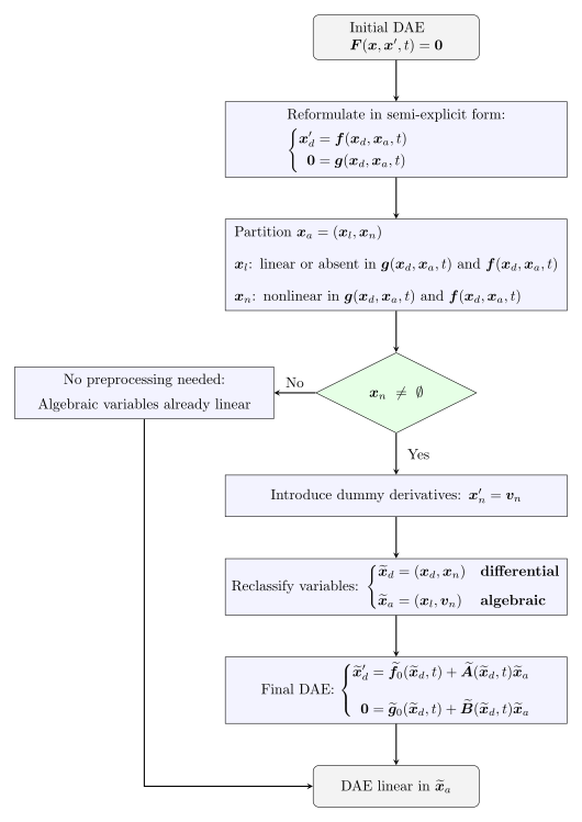
The index reduction algorithm now work as for the index reduction for nonlinear DAE (see Section 13.4) but working with the matrix \bm{B}(\bm{x}_d,t).
Step 1: Check if \bm{B}(\bm{x}_d,t) is Singular
The constraints are written as:
\bm{B}(\bm{x}_d,t) \bm{x}_a = -\bm{g}(\bm{x}_d,t),
Compute the determinant:
If \det(\bm{B}(\bm{x}_d,t)) \neq 0, then \bm{B}(\bm{x}_d,t) is invertible
the DAE is of index 1: \bm{x}_a = -\bm{B}(\bm{x}_d,t)^{-1}\bm{g}(\bm{x}_d,t)
Terminate the procedure.
If \det(\bm{B}(\bm{x}_d,t)) = 0
\bm{B}(\bm{x}_d,t) is singular
the DAE is of index >1.
Proceed to the next step.
Step 2: Decompose the linear system
Determine the rank of \bm{B}(\bm{x}_d,t), denoted as r = \operatorname{rank}(\bm{B}) and define:
A basis \bm{Q}_a(\bm{x},t) \in \Bbb{R}^{n_a \times (n_a-k)} for the null space \mathcal{N}(\bm{B}(\bm{x},t)^T), which identifies the algebraic constraints that can be differentiated. This basis satisfies:
\bm{B}(\bm{x}_d,t)^T\bm{Q}_a(\bm{x}_d,t) = \bm{0} or equivalently
\bm{Q}_a(\bm{x}_d,t)^T\bm{B}(\bm{x}_d,t) = \bm{0}.
A matrix \bm{Q}_d(\bm{x}_d,t) \in \Bbb{R}^{n_a \times k} that completes \bm{Q}_a(\bm{x}_d,t) to a full basis, ensuring that: \bm{Q}(\bm{x}_d,t) = \begin{pmatrix} \bm{Q}_d(\bm{x}_d,t), \bm{Q}_a(\bm{x}_d,t) \end{pmatrix} is non-singular.
By multiplying the original constraints by \bm{Q}(\bm{x}_d,t)^T, we obtain:
Part that contains \bm{x}_a: \color{blue} \bm{B}_d(\bm{x}_d,t) \bm{x}_a = -\bm{g}_d(\bm{x}_d,t), where: \begin{aligned} \bm{B}_d(\bm{x}_d,t) &= \bm{Q}_d(\bm{x}_d,t)^T \bm{B}(\bm{x}_d,t), \\ \bm{g}_d(\bm{x}_d,t) &= \bm{Q}_d(\bm{x}_d,t)^T\bm{g}(\bm{x}_d,t). \end{aligned}
Part free of \bm{x}_a: \color{blue} \bm{g}_a(\bm{x},t) = \bm{0}, where: \bm{g}_a(\bm{x}_d,t) = \bm{Q}_a(\bm{x}_d,t)^T\bm{g}(\bm{x}_d,t). Since \bm{Q}_a(\bm{x}_d,t)^T \bm{B}(\bm{x}_d,t) = \bm{0}, no algebraic variables appear in this equation.
Step 4: Differentiate the Algebraic Constraints
The algebraic constraints must be differentiated to reveal hidden differential equations:
\frac{\mathrm{d}}{\mathrm{d}t} \bm{g}_a(\bm{x}_d,t) = \dfrac{\partial\bm{g}_a(\bm{x}_d,t)}{\partial t} + \dfrac{\partial\bm{g}_a(\bm{x}_d,t)}{\partial\bm{x}_d} \bm{x}_d^\prime(t) = \bm{0}.
Rewriting, the constraints becomes:
\begin{pmatrix} \bm{B}_d(\bm{x}_d,t) \\[1em] \dfrac{\partial\bm{g}_a(\bm{x}_d,t)}{\partial\bm{x}_d} \end{pmatrix} \bm{x}_d^\prime = - \begin{pmatrix} \bm{g}_d(\bm{x}_d,t) \\[1em] \dfrac{\partial\bm{g}_a(\bm{x}_d,t)}{\partial t} \end{pmatrix}.
and using \bm{x}'_d = \bm{f}(\bm{x}_d,t) + \bm{A}(\bm{x}_d,t)\bm{x}_a can be rewritten as
\begin{pmatrix} \bm{B}_d(\bm{x}_d,t) \\[1em] \dfrac{\partial\bm{g}_a(\bm{x}_d,t)}{\partial\bm{x}_d} \end{pmatrix} \bm{A}(\bm{x}_d,t)\bm{x}_a = - \begin{pmatrix} \bm{g}_d(\bm{x}_d,t) \\[1em] \dfrac{\partial\bm{g}_a(\bm{x}_d,t)}{\partial t} \end{pmatrix} - \begin{pmatrix} \bm{B}_d(\bm{x}_d,t) \\[1em] \dfrac{\partial\bm{g}_a(\bm{x}_d,t)}{\partial\bm{x}_d} \end{pmatrix} \bm{f}(\bm{x}_d,t)
or better
\begin{pmatrix} \bm{B}_d(\bm{x}_d,t) \\[1em] \dfrac{\partial\bm{g}_a(\bm{x}_d,t)}{\partial\bm{x}_d} \end{pmatrix} \bm{A}(\bm{x}_d,t) \bm{x}_a = - \begin{pmatrix} \bm{g}_d(\bm{x}_d,t) + \bm{B}_d(\bm{x}_d,t)\bm{f}(\bm{x}_d,t) \\[1em] \dfrac{\partial\bm{g}_a(\bm{x}_d,t)}{\partial t} +\dfrac{\partial\bm{g}_a(\bm{x}_d,t)}{\partial\bm{x}_d}\bm{f}(\bm{x}_d,t) \end{pmatrix}
Defining:
\begin{aligned} \widetilde{\bm{B}}(\bm{x}_d,t) &= \begin{pmatrix} \bm{B}_d(\bm{x}_d,t) \\[1em] \dfrac{\partial\bm{g}_a(\bm{x}_d,t)}{\partial\bm{x}_d} \end{pmatrix} \bm{A}(\bm{x}_d,t), \\ \widetilde{\bm{g}}(\bm{x}_d,t) &= \begin{pmatrix} \bm{g}_d(\bm{x}_d,t) + \bm{B}_d(\bm{x}_d,t)\bm{f}(\bm{x}_d,t) \\[1em] \dfrac{\partial\bm{g}_a(\bm{x}_d,t)}{\partial t} +\dfrac{\partial\bm{g}_a(\bm{x}_d,t)}{\partial\bm{x}_d}\bm{f}(\bm{x}_d,t) \end{pmatrix} \end{aligned}
we obtain a new constraint part of the DAE:
\widetilde{\bm{B}}(\bm{x}_d,t) \bm{x}_a = -\widetilde{\bm{g}}(\bm{x}_d,t).
notice that the DAE is still in the form with linear algebraic constraints.
Go to step 1.
The differentiation index is the number of times Step 4 is performed plus one before reaching an index 1 DAE.