
12 Index reduction of a Linear DAE
A Differential-Algebraic Equation (DAE) is a system of equations that consists of both differential and algebraic equations. Unlike ordinary differential equations (ODEs), DAEs may contain constraints that restrict the solution space. The (differential) index of a DAE measures how many times the system must be differentiated to convert it into an explicit ODE.
This tutorial explains how to compute the index of a linear DAE systematically, assuming constant coefficient matrices and avoiding the Kronecker canonical form.
12.1 Steps to Compute the Index
First recall that a linear DAE with constant coefficients is given by:
\bm{E} \bm{x}^\prime + \bm{A} \bm{x} = \bm{f}(t)
where:
- \bm{E} and \bm{A} are constant matrices,
- \bm{x}(t) is the state variable,
- \bm{f}(t) is an input function,
- \bm{x}^\prime is the time derivative of \bm{x}.
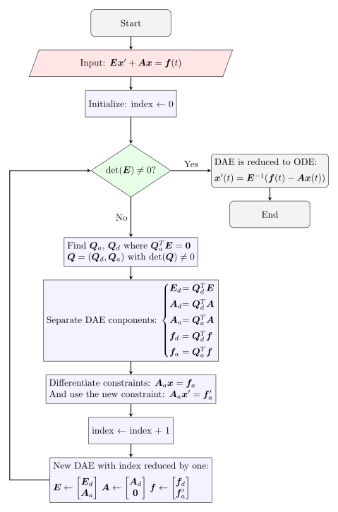
The following steps provide a rough outline of the approach, offering a general understanding of the index reduction procedure.
Step 1: Check if \bm{E} is Singular
Compute \det(\bm{E}):
If \det(\bm{E}) \neq 0, then \bm{E} is invertible, and the system reduces to an ODE (index 0). Terminate procedure.
If \det(\bm{E}) = 0, then \bm{E} is singular, indicating the presence of algebraic constraints. Proceed to the next step.
Step 2: Decompose the System into Differential and Algebraic Parts
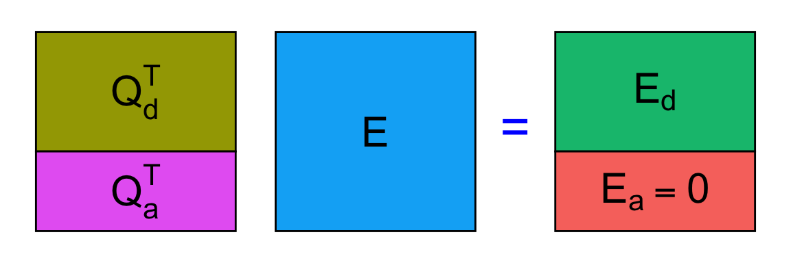
Determine the rank of \bm{E}\in\Bbb{R}^{n\times n}, denoted as r = \operatorname{rank}(\bm{E}). Find:
A basis \bm{Q}_a\in\Bbb{R}^{n\times (n-k)} for the null space \mathcal{N}(\bm{E}^T), which identifies the algebraic constraints.
The basis satisfy \bm{E}^T\bm{Q}_a=\bm{0} or transposing \bm{Q}_a^T\bm{E}=\bm{0}.A matrix \bm{Q}_d\in\Bbb{R}^{n\times k} that complete \bm{Q}_a to a basis. In practice \bm{Q}_d make the matrix \bm{Q}=(\bm{Q}_d,\bm{Q}_a) non singular.
Decomposing the system: \bm{E} \bm{x}^\prime + \bm{A} \bm{x} = \bm{f}(t) by multiplying to the left with \bm{Q}^T:
Differential part: \bm{E}_d \bm{x}^\prime + \bm{A}_d\bm{x} = \bm{f}_d(t) where \bm{E}_d=\bm{Q}_d^T \bm{E}, \quad \bm{A}_d = \bm{Q}_d^T\bm{A}, \quad \bm{f}_d(t) = \bm{Q}_d^T\bm{f}(t)
Algebraic part: \bm{A}_a \bm{x} = \bm{f}_a(t) where \bm{A}_a = \bm{Q}_a^T\bm{A}, \qquad \bm{f}_a(t) = \bm{Q}_a^T\bm{f}(t)
since \bm{Q}_a^T \bm{E} = \bm{0}.
Remark 12.1. The decomposition used to separate differential and algebraic part seem quite cumbersome and difficult at first. However, in practice, it is straightforward to compute using standard tools from linear algebra. For instance, the LU decomposition can be applied to the matrix \bm{E} to efficiently compute \bm{Q}_A and \bm{Q}_b. The detail will be discussed forward.
Step 3: Handle the Algebraic Constraints
The algebraic constraints from Step 2 are:
\bm{A}_a \bm{x} = \bm{f}_a(t)).
Differentiate these constraints:
\bm{A}_a \bm{x}^\prime = \bm{f}_a^\prime (t)
Now the DAE take the form
\begin{pmatrix} \bm{E}_d \\ \bm{A}_a \end{pmatrix} \bm{x}^\prime + \begin{pmatrix} \bm{A}_d \\ \bm{0} \end{pmatrix} \bm{x} = \begin{pmatrix} \bm{f}_d(t) \\ \bm{f}_a^\prime(t) \end{pmatrix}
or
\widetilde{\bm{E}} \bm{x}^\prime + \widetilde{\bm{A}} \bm{x} = \widetilde{\bm{f}}(t)
where
\widetilde{\bm{E}}= \begin{pmatrix} \bm{E}_d \\ \bm{A}_a \end{pmatrix} \quad \widetilde{\bm{A}}= \begin{pmatrix} \bm{A}_d \\ \bm{0} \end{pmatrix} \quad \widetilde{\bm{f}}(t)= \begin{pmatrix} \bm{f}_d(t) \\ \bm{f}_a^\prime(t) \end{pmatrix}
Return to step 1. When termninate the procedure the index is the number of time Step 3 (differentiation) is performed.
12.2 Practical construction of \bm{Q}_a and \bm{Q}_d
For the systematic construction of the matrices \bm{Q}_a and \bm{Q}_d, we leverage the (generalized) LU decomposition, which provides a structured way to separate the differential and algebraic components of a Differential-Algebraic Equation (DAE).
Theorem 12.1 (see [1], [2]) Let \bm{A}\in\Bbb{R}^{n \times m} of rank k\leqslant\min(n,m), then there exists two permutation matrices \bm{P}_L and \bm{P}_R such that
\bm{P}_L\bm{A}\bm{P}_R = \begin{pmatrix} \bm{L} & \bm{0} \\ \bm{M} & \bm{I} \end{pmatrix} \begin{pmatrix} \bm{U} & \bm{N} \\ \bm{0} & \bm{0} \end{pmatrix}
with
- \bm{L}\in\Bbb{R}^{k\times k} lower triangular with 1 on the main diagonal.
- \bm{U}\in\Bbb{R}^{k\times k} upper triangular with nonzero element on the main diagonal.
- \bm{M}\in\Bbb{R}^{{n-k}\times k}
- \bm{N}\in\Bbb{R}^{k\times {m-k}}
Using this theorem for \bm{E}:
\bm{P}_L\,\bm{E}\,\bm{P}_R = \begin{pmatrix} \bm{L} & \bm{0} \\ \bm{M} & \bm{I} \end{pmatrix} \begin{pmatrix} \bm{U} & \bm{N} \\ \bm{0} & \bm{0} \end{pmatrix}
and (using the fact that for a permutation matrix \bm{P}^{-1}=\bm{P}^T)
\bm{E} = \bm{P}_L^T \begin{pmatrix} \bm{L} & \bm{0} \\ \bm{M} & \bm{I} \end{pmatrix} \begin{pmatrix} \bm{U} & \bm{N} \\ \bm{0} & \bm{0} \end{pmatrix} \bm{P}_R^T
so that defining
\bm{Q}^T = \begin{pmatrix} \bm{L} & \bm{0} \\ \bm{M} & \bm{I} \end{pmatrix}^{-1} \bm{P}_L = \begin{pmatrix} \bm{L}^{-1} & \bm{0} \\ -\bm{M}\bm{L}^{-1} & \bm{I} \end{pmatrix} \bm{P}_L
we have
\begin{aligned} \bm{Q}^T\bm{E}& = \underbrace{ \begin{pmatrix} \bm{L}^{-1} & \bm{0} \\ -\bm{M}\bm{L}^{-1} & \bm{I} \end{pmatrix} \bm{P}_L }_{\bm{Q}^T} \;\; \underbrace{ \bm{P}_L^T \begin{pmatrix} \bm{L} & \bm{0} \\ \bm{M} & \bm{I} \end{pmatrix} \begin{pmatrix} \bm{U} & \bm{N} \\ \bm{0} & \bm{0} \end{pmatrix} \bm{P}_R^T }_{\bm{E}} \\[1em] & = \begin{pmatrix} \bm{U} & \bm{N} \\ \bm{0} & \bm{0} \end{pmatrix} \bm{P}_R^T \end{aligned}
Simplification
we can discard the colum permutation \bm{P}_R defining
\begin{pmatrix} \bm{E}_d \\ \bm{0} \end{pmatrix} = \begin{pmatrix} \bm{U} & \bm{N} \\ \bm{0} & \bm{0} \end{pmatrix} \bm{P}_R^T
so that
\bm{E} = \bm{P}_L^T \begin{pmatrix} \bm{L} & \bm{0} \\ \bm{M} & \bm{I} \end{pmatrix} \begin{pmatrix} \bm{S} \\ \bm{0} \end{pmatrix}, \quad \bm{Q}^T \bm{E} = \begin{pmatrix} \bm{E}_d \\ \bm{0} \end{pmatrix},
and applying \bm{Q}^T to the DAE \bm{E} \bm{x}^\prime + \bm{A} \bm{x} = \bm{f}(t) results in
\begin{aligned} \bm{Q}^T\left( \bm{E}\,\bm{x}^\prime+\bm{A}\,\bm{x} \right) &=\bm{Q}^T\bm{f}(t) \\[1em] \begin{pmatrix} \bm{E}_d \\ \bm{0} \end{pmatrix} \bm{x}^\prime +\bm{Q}^T\bm{A}\bm{x} &= \bm{Q}^T\bm{f}(t) \end{aligned}
and there is a practical separation of the algebraic equation from the DAE.
Remark 12.2 (Avoiding explicit construction of \bm{Q}_a and \bm{Q}_d). The separation of differential and algebraic part is equivalent to the reduction to echelon form (see Chapter 8). This method is a systematic approach to solving linear systems, computing ranks, and checking singularity conditions.
12.3 Index Reduction Algorithm for linear DAEs
12.4 Example 1
Index Reduction of a Linear DAE
Consider the following linear DAE:
\begin{aligned} x_1^\prime + x_2 & = 0, \\ x_1 & = 1, \end{aligned}
That written in matrix form become:
\bm{E} \bm{x}^\prime + \bm{A} \bm{x} = \bm{f}(t),
with the following matrices and vectors:
\bm{E} = \begin{bmatrix} 1 & 0 \\ 0 & 0 \end{bmatrix}, \quad \bm{A} = \begin{bmatrix} 0 & 1 \\ 1 & 0 \end{bmatrix}, \quad \bm{f}(t) = \begin{bmatrix} 0 \\ 1 \end{bmatrix}.
First reduction
Step 1: Check if \bm{E} is Singular
We compute:
\det(\bm{E}) = 0
Since \bm{E} is singular, the system is a DAE.
Step 2: Decompose the System
The basis for the null space of \bm{E}^T is: \bm{Q}_a =\begin{bmatrix}0 \\1\end{bmatrix}.
The complementary vector is: \bm{Q}_d =\begin{bmatrix} 1 \\ 0 \end{bmatrix}.
We construct the matrix \bm{Q} =\begin{bmatrix}1 & 0 \\0 & 1\end{bmatrix}.
Multiplying the system by \bm{Q}^T, we get the new matrices:
\begin{aligned} \bm{E}_d &= \bm{Q}_d^T \bm{E} &=& \begin{bmatrix} 1 & 0 \end{bmatrix} \begin{bmatrix} 1 & 0 \\ 0 & 0 \end{bmatrix} &=& \begin{bmatrix} 1 & 0 \end{bmatrix}, \\ \bm{A}_d & = \bm{Q}_d^T\bm{A} &=& \begin{bmatrix} 1 & 0 \end{bmatrix} \begin{bmatrix} 0 & 1 \\ 1 & 0 \end{bmatrix} &=& \begin{bmatrix} 0 & 1 \end{bmatrix}, \\ \bm{f}_d(t) & = \bm{Q}_d^T \bm{f}(t) &=& \begin{bmatrix} 1 & 0 \end{bmatrix} \begin{bmatrix} 0 \\ 1 \end{bmatrix} &=& \begin{bmatrix} 0 \end{bmatrix}, \\ \bm{A}_a & = \bm{Q}_a^T \bm{A} &=& \begin{bmatrix} 0 & 1 \end{bmatrix} \begin{bmatrix} 0 & 1 \\ 1 & 0 \end{bmatrix} &=& \begin{bmatrix} 1 & 0 \end{bmatrix}, \\ \bm{f}_a(t) & = \bm{Q}_a^T \bm{f}(t) &=& \begin{bmatrix} 0 & 1 \end{bmatrix} \begin{bmatrix} 0 \\ 1 \end{bmatrix} &=& \begin{bmatrix} 1 \end{bmatrix}. \end{aligned}
Step 3: Solve the System
The system becomes:
Differential part: x_1^\prime + x_2 = 0.
Algebraic part: x_1 = 1.
Differentiating the algebraic constraint x_1 = 1:
x_1^\prime = 0.
At this point the DAE become:
\widetilde{\bm{E}} \bm{x}^\prime + \widetilde{\bm{A}} \bm{x} = \widetilde{\bm{f}}(t)
with the following matrices and vectors:
\widetilde{\bm{E}} = \begin{bmatrix} 1 & 0 \\ 1 & 0 \end{bmatrix}, \quad \widetilde{\bm{A}} = \begin{bmatrix} 0 & 1 \\ 0 & 0 \end{bmatrix}, \quad \widetilde{\bm{f}}(t) = \begin{bmatrix} 0 \\ 0 \end{bmatrix}.
Second Reduction
Now reapply the algorithm:
Step 1: Check if \widetilde{\bm{E}} is Singular
We compute:
\det(\widetilde{\bm{E}}) = 0
Since \widetilde{\bm{E}} is singular, the system is still a DAE.
Step 2: Decompose the System
The basis for the null space of \widetilde{\bm{E}}^T is: \widetilde{\bm{Q}}_a =\begin{bmatrix} 1 \\ -1 \end{bmatrix}.
The complementary vector is: \widetilde{\bm{Q}}_d =\begin{bmatrix} 1 \\ 1 \end{bmatrix}.
We construct the matrix \widetilde{\bm{Q}} =\begin{bmatrix} 1 & 1 \\ 1 & -1 \end{bmatrix}.
Multiplying the system by \widetilde{\bm{Q}}^T, we get the new matrices:
\begin{aligned} \widetilde{\bm{E}}_d &= \widetilde{\bm{Q}}_d^T \widetilde{\bm{E}} &=& \begin{bmatrix} 1 & 1 \end{bmatrix} \begin{bmatrix} 1 & 0 \\ 1 & 0 \end{bmatrix} &=& \begin{bmatrix} 2 & 0 \end{bmatrix}, \\ \widetilde{\bm{A}}_d &= \widetilde{\bm{Q}}_d^T \widetilde{\bm{A}} &=& \begin{bmatrix} 1 & 1 \end{bmatrix} \begin{bmatrix} 0 & 1 \\ 0 & 0 \end{bmatrix} &=& \begin{bmatrix} 0 & 1 \end{bmatrix}, \\ \widetilde{\bm{f}}_d(t) &= \widetilde{\bm{Q}}_d^T \widetilde{\bm{f}(}t) &=& \begin{bmatrix} 1 & 1 \end{bmatrix} \begin{bmatrix} 0 \\ 0 \end{bmatrix} &=& \begin{bmatrix} 0 \end{bmatrix}, \\ \widetilde{\bm{A}}_a &= \widetilde{\bm{Q}}_a^T\widetilde{\bm{A}} &=& \begin{bmatrix} 1 & -1 \end{bmatrix} \begin{bmatrix} 0 & 1 \\ 0 & 0 \end{bmatrix} &=& \begin{bmatrix} 0 & 1 \end{bmatrix}, \\ \widetilde{\bm{f}}_a(t) &= \widetilde{\bm{Q}}_a^T \widetilde{\bm{f}}(t) &=& \begin{bmatrix} 1 & -1 \end{bmatrix} \begin{bmatrix} 0 \\ 0 \end{bmatrix} &=& \begin{bmatrix} 0 \end{bmatrix}. \end{aligned}
Step 3: Solve the System
The system becomes:
Differential part: 2x_1^\prime + x_2 = 0.
Algebraic part: x_2 = 0.
Differentiating the algebraic constraint x_2 = 0:
x_2^\prime = 0.
At this point the DAE become:
\widetilde{\widetilde{\bm{E}}} \bm{x}^\prime + \widetilde{\widetilde{\bm{A}}} \bm{x} = \widetilde{\widetilde{\bm{f}}}(t)
with the following matrices and vectors:
\widetilde{\widetilde{\bm{E}} } = \begin{bmatrix} 2 & 0 \\ 0 & 1 \end{bmatrix}, \quad \widetilde{\widetilde{\bm{A}}} = \begin{bmatrix} 0 & 1 \\ 0 & 0 \end{bmatrix}, \quad \widetilde{\widetilde{\bm{f}}}(t) = \begin{bmatrix} 0 \\ 0 \end{bmatrix}.
Now reapply the algorithm. At the step 1 \det( \widetilde{\widetilde{\bm{E}}} )=2\neq 0 so now we have an ODE:
\begin{aligned} 2x_1^\prime + x_2 &= 0, \\ x_2^\prime &= 0. \end{aligned}
we have done two derivation, thus the index of original DAE is 2.
12.5 Example 2
Consider the DAE
\left\{ \begin{aligned} x'(t) &= z(t)\\ z'(t) &= y(t)-t \\ x'(t) &= z(t)+x(t)+t+1 \end{aligned} \right.
define
\bm{E} = \begin{pmatrix} 1 & 0 & 0 \\ 0 & 0 & 1 \\ 1 & 0 & 0 \end{pmatrix}, \qquad \bm{A} = \begin{pmatrix} 0 & 0 & -1 \\ 0 & -1 & 0 \\ -1 & 0 & -1 \end{pmatrix}, \qquad \bm{f}(t) = \begin{pmatrix} 0 \\ -t \\ t+1 \end{pmatrix}
so that the DAE can be written as
\bm{E}\,\bm{x}^\prime(t) + \bm{A}\,\bm{x}(t) = \bm{f}(t)
The table
\bm{T} = \left[\begin{array}{c|c|c} \bm{E} & \bm{A} & \bm{f}(t) \end{array} \right] = \left[ \begin{array}{rrr|rrr|c} 1 & 0 & 0 & 0 & 0 & -1 & 0 \\ 0 & 0 & 1 & 0 & -1 & 0 & -t \\ 1 & 0 & 0 & -1 & 0 & -1 & t+1 \end{array} \right]
is used to memorize the operation done on the DAE. Let \textrm{index}\leftarrow 0.
Multiply table \bm{T} on the left by \bm{L}_1 where
\bm{L}_1 = \begin{pmatrix} 1 & 0 & 0 \\ 0 & 1 & 0 \\ -1 & 0 & 1 \end{pmatrix}
so that
\bm{T}_1 = \bm{L}_1\bm{T} = \left[ \begin{array}{rrr|rrr|c} 1 & 0 & 0 & 0 & 0 & -1 & 0 \\ 0 & 0 & 1 & 0 & -1 & 0 & -t \\ \hline \color{red}0 & \color{red}0 & \color{red}0 & \color{red}-1 & \color{red}0 & \color{red}0 & \color{red}t+1 \end{array} \right]
The last row contain the algebraic equation
\color{blue} -x(t) = t+1
First block now is in echelon form. Apply derivation of the last row (reduce index by one). Let \textrm{index}\leftarrow 1.
\bm{T}_2 = \left[ \begin{array}{rrr|rrr|c} 1 & 0 & 0 & 0 & 0 & -1 & 0 \\ 0 & 0 & 1 & 0 & -1 & 0 & -t \\ \hline \color{red}-1 & \color{red}0 & \color{red}0 & \color{red}0 & \color{red}0 & \color{red}0 & \color{red}1 \end{array} \right]
Multiply table \bm{T}_2 on the left by \bm{L}_2 where
\bm{L}_2 = \begin{pmatrix} 1 & 0 & 0 \\ 0 & 1 & 0 \\ 1 & 0 & 1 \end{pmatrix}
so that
\bm{T}_3 = \bm{L}_2\bm{T}_2 = \left[ \begin{array}{rrr|rrr|c} 1 & 0 & 0 & 0 & 0 & -1 & 0 \\ 0 & 0 & 1 & 0 & -1 & 0 & -t \\ \hline \color{red} 0 & \color{red}0 & \color{red}0 & \color{red}0 & \color{red}0 & \color{red}-1 & \color{red}1 \end{array} \right]
The last row contain the algebraic equation
\color{blue} -z(t) = 1
First block again is in echelon form. Apply derivation of the last row (reduce index by one). Let \textrm{index}\leftarrow 2.
\bm{T}_4 = \left[ \begin{array}{rrr|rrr|c} 1 & 0 & 0 & 0 & 0 & -1 & 0 \\ 0 & 0 & 1 & 0 & -1 & 0 & -t \\ \hline \color{red}0 & \color{red}0 & \color{red}-1 & \color{red} 0 & \color{red}0 & \color{red}0 & \color{red}0 \end{array} \right]
Multiply table \bm{T}_4 on the left by \bm{L}_4 where
\bm{L}_4 = \begin{pmatrix} 1 & 0 & 0 \\ 0 & 1 & 0 \\ 0 & 1 & 1 \end{pmatrix}
so that
\bm{T}_5 = \bm{L}_4\bm{T}_4 = \left[ \begin{array}{rrr|rrr|c} 1 & 0 & 0 & 0 & 0 & -1 & 0 \\ 0 & 0 & 1 & 0 & -1 & 0 & -t \\ \hline \color{red}0 & \color{red}0 & \color{red}0 & \color{red} 0 & \color{red}-1 & \color{red}0 & \color{red}-t \end{array} \right]
The last row contain the algebraic equation
\color{blue} -y(t) = -t
First block again is in echelon form. Apply derivation of the last row (reduce index by one). Let \textrm{index}\leftarrow 3.
\bm{T}_6 = \left[ \begin{array}{rrr|rrr|c} 1 & 0 & 0 & 0 & 0 & -1 & 0 \\ 0 & 0 & 1 & 0 & -1 & 0 & -t \\ \hline \color{red} 0 & \color{red}-1 & \color{red}0 & \color{red}0 & \color{red}0 & \color{red}0 & \color{red}-1 \end{array} \right]
Exchange last two rows and multily by -1 second row
\bm{P}_6 = \begin{pmatrix} 1 & 0 & 0 \\ 0 & 0 & -1 \\ 0 & 1 & 0 \end{pmatrix}
multilying \bm{T}_6 by \bm{P}_6:
\bm{P}_6\bm{T}_6 = \left[ \begin{array}{rrr|rrr|c} 1 & 0 & 0 & 0 & 0 & -1 & 0 \\ 0 & 1 & 0 & 0 & 0 & 0 & 1 \\ 0 & 0 & 1 & 0 & -1 & 0 & -t \end{array} \right]
The ODE after index reduction \left\{ \begin{aligned} x'(t) &= z(t)\\ y'(t) &= 1 \\ z'(t) &= y(t)-t \end{aligned} \right.
The algebraic (hidden) constraints
\begin{aligned} -x(t) & = t+1 \\ -z(t) & = 1 \\ -y(t) & = -t \end{aligned} \implies \left\{ \begin{aligned} x(t) & = -t-1 \\ z(t) & = -1 \\ y(t) & = t \end{aligned} \right.
The differential index is 3
Notice that the hiddent constaints determine the complete solution and the initial condition of the ODE (x(0),y(0),z(0))=(-1,-1,0).
12.6 Example 3
Consider the DAE
\left\{ \begin{aligned} x'(t) &= z(t)\\ x'(t) &= y(t)-\sin t \\ x'(t) &= z(t)+y(t)+ \cos t \end{aligned} \right.
define
\bm{E} = \begin{pmatrix} 1 & 0 & 0 \\ 1 & 0 & 0 \\ 1 & 0 & 0 \end{pmatrix}, \qquad \bm{A} = \begin{pmatrix} 0 & 0 & -1 \\ 0 & -1 & 0 \\ 0 & -1 & -1 \end{pmatrix}, \qquad \bm{f}(t) = \begin{pmatrix} 0 \\ -\sin t \\ \cos t \end{pmatrix}
so that the DAE can be written as
\bm{E}\,\bm{x}^\prime(t) + \bm{A}\,\bm{x}(t) = \bm{f}(t)
The table
\bm{T} = \left[\begin{array}{c|c|c} \bm{E} & \bm{A} & \bm{f}(t) \end{array} \right] = \left[ \begin{array}{rrr|rrr|c} 1 & 0 & 0 & 0 & 0 & -1 & 0 \\ 1 & 0 & 0 & 0 & -1 & 0 & -\sin t \\ 1 & 0 & 0 & 0 & -1 & -1 & \cos t \end{array} \right]
is used to memorize the operation done on the DAE. Let \textrm{index}\leftarrow 0.
Multiply table \bm{T} on the left by \bm{L}_1 where
\bm{L}_1 = \begin{pmatrix} 1 & 0 & 0 \\ -1 & 1 & 0 \\ -1 & 0 & 1 \end{pmatrix}
so that
\bm{T}_1 = \bm{L}_1\bm{T} = \left[ \begin{array}{rrr|rrr|c} 1 & 0 & 0 & 0 & 0 & -1 & 0 \\ \hline \color{red}0 & \color{red}0 & \color{red}0 & \color{red}0 & \color{red}-1 & \color{red}+1 & \color{red}-\sin t \\ \color{red}0 & \color{red}0 & \color{red}0 & \color{red}0 & \color{red}-1 & \color{red} 0 & \color{red}\cos t \end{array} \right]
The last two rows contains the algebraic equations
\color{blue} -y(t)+z(t) = -\sin t, \qquad -y(t)=\cos(t)
First block now is in echelon form. Apply derivation of the last rows (reduce index by one). Let \textrm{index}\leftarrow 1.
\bm{T}_2 = \left[ \begin{array}{rrr|rrr|c} 1 & 0 & 0 & 0 & 0 & -1 & 0 \\ \hline \color{red}0 & \color{red}-1 & \color{red}+1 & \color{red}0 & \color{red}0 & \color{red}0 & \color{red}-\cos t \\ \color{red}0 & \color{red}-1& \color{red} 0 & \color{red}0 & \color{red}0 & \color{red}0 & \color{red}-\sin t \end{array} \right]
Multiply table \bm{T}_2 on the left by \bm{L}_2 where
\bm{L}_2 = \begin{pmatrix} 1 & 0 & 0 \\ 0 & 1 & 0 \\ 0 & -1 & 1 \end{pmatrix}
so that
\bm{T}_3 = \bm{L}_2\bm{T}_2 = \left[ \begin{array}{rrr|rrr|c} 1 & 0 & 0 & 0 & 0 & -1 & 0 \\ 0 & -1 & +1 & 0 & 0 & 0 & -\cos t \\ 0 & 0 & -1 & 0 & 0 & 0 & \cos t-\sin t \end{array} \right]
The ODE after index reduction
\begin{aligned} x'(t) & = z(t) \\ -y'(t)+z'(t) & = -\cos t \\ -z'(t) & = \cos t - \sin t \end{aligned} \implies \left\{ \begin{aligned} x'(t) & = z(t) \\ y'(t) & = \sin t \\ z'(t) & = \sin t - \cos t \end{aligned} \right.
The algebraic (hidden) constraints
\begin{aligned} -y(t)+z(t) &= -\sin t, \\ -y(t) &= \cos t \end{aligned} \implies \left\{ \begin{aligned} y(t) & = -\cos t \\ z(t) & = \cos t - \sin t \end{aligned} \right.
The differential index is 2
Notice that the hiddent constaints determine part of complete solution and the initial condition of the ODE (x(0),y(0),z(0))=(\textrm{free},-1,0). Thus, only z(0) must be set to determine the solution.