22 Coordinate Partitioning for Pendulum in cartesian coordinates

22.1 Step 1 choose independent coordinates
Consider redundant coordinate pendulum DAE
\begin{aligned} u^{\prime} &= \mu x\\ v^{\prime} &= \mu y-g\\ x^{\prime} &= u \\ y^{\prime} &= v \\ x^2+y^2 &= r^2 \end{aligned}
Solve y as a function of x (use negative branch)
\color{blue}y(x) = -\sqrt{r^2-x^2}
constraint can be eliminated from the DAE by introducing y\equiv y(x).
22.2 Step 2a propagate constraints
\begin{aligned} u^{\prime} &= \mu x\\ v^{\prime} &= \mu {\color{blue}y(x)}-g\\ x^{\prime} &= u \\ y^{\prime} &= v \\ \color{blue}y(x) &\color{blue}=-\sqrt{r^2-x^2} \end{aligned}
Deriving constraint x^2+y^2-r^2=0 derivative of y^{\prime}(x) is deduced
x\dot{x}+y\dot{y} = 0\quad\Longrightarrow\quad \dot{y} = -x\dot{x}/y\quad\Longrightarrow\quad v = -xu/y
so that
\color{red}\dot{y}=v(x,u) = -\frac{xu}{y(x)}
22.3 Step 2b propagate constraints
Substitute \dot{y} with v(x,u)
\begin{aligned} u^{\prime} &= \mu x\\ v^{\prime} &= \mu {\color{blue}y(x)}-g\\ x^{\prime} &= u \\ \color{red}v(x,u)&\color{red}=-\frac{xu}{y(x)}\\ \color{blue}y(x) &\color{blue}=-\sqrt{r^2-x^2} \end{aligned}
22.4 Step 2c propagate constraints
Deriving two time the constraint x^2+y^2-r^2=0 derivative \ddot{y}=\dot{v} is deduced:
\begin{aligned} x u^{\prime}+y\dot{v}+ x^{\prime}u+y^{\prime}v&=0\quad\Longrightarrow\\[1em] \mu (x^2+y^2)-gy+(u^2+v^2)&=0 \end{aligned}
so that \mu can be written as a function of x and u
\color{purple}\mu(x,u) =\frac{gy(x)- (u^2+v(x,u)^2) } {r^2}
thus \mu=\mu(x,u) and
v^{\prime}(x,u)={\color{purple}\mu(x,u)} {\color{blue}y(x)}-g
can be eliminated as redundant algebraic equation.
22.5 Step 2d propagate constraints
Substitute \mu=\mu(x,u)
\begin{aligned} u^{\prime}&={\color{purple}\mu(x,u)} x\\ %\dot{v}&=&{\color{purple}\mu(x,u)} {\color{blue}y(x)}-g\\ x^{\prime}&=u \\ \color{purple}\mu(x,u) &\color{purple}=\frac{gy(x)- (u^2+v(x,u)^2) } {r^2}\\ \color{red}v(x,u)&\color{red}=-\frac{xu}{y(x)}\\ \color{blue}y(x) &\color{blue}=-\sqrt{r^2-x^2} \end{aligned}
in practice an ODE with 2 equations and \mu(x,u) computed recursively.
22.6 Collatz
Using Collatz explicit integrator
\begin{aligned} u_{k+1/2}&=u_k+(h/2)\mu(x_k,u_k)x_k\\ x_{k+1/2}&=x_k+(h/2)u_k \\[1em] u_{k+1}&=u_k+h\,\mu(x_{k+1/2},u_{k+1/2})x_{k+1/2}\\ x_{k+1}&=x_k+h\,u_{k+1/2} \end{aligned}
where \mu(x,u)
\begin{aligned} \color{red}y_k &= -\sqrt{r^2-x_k^2} \\ \color{red}v_k &= -\frac{x_ku_k}{\color{red}y_k}\\ \mu(x_k,u_k) &= \frac{g{\color{red}y_k}- (u_k^2+{\color{red}v_k}^2) } {r^2} \end{aligned}
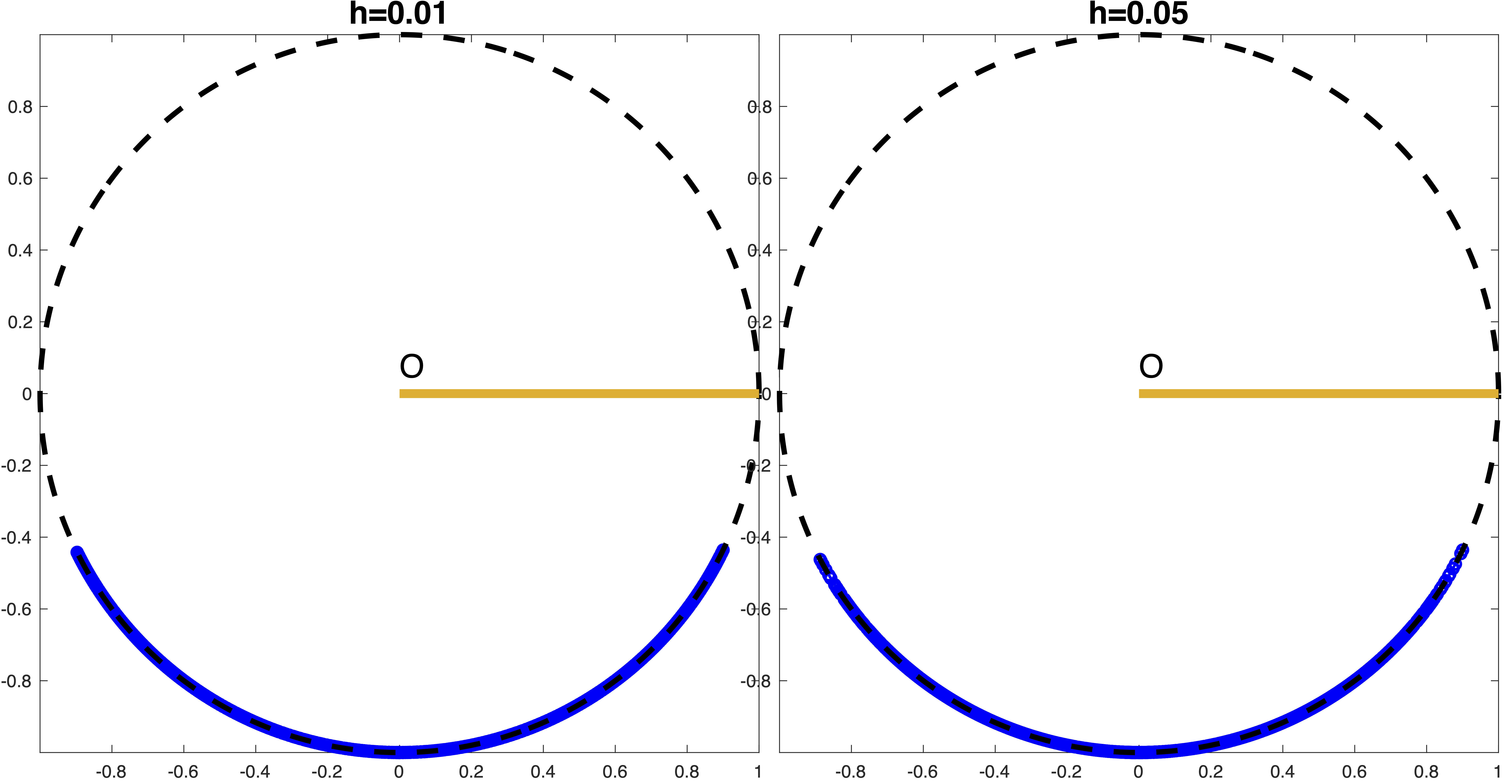
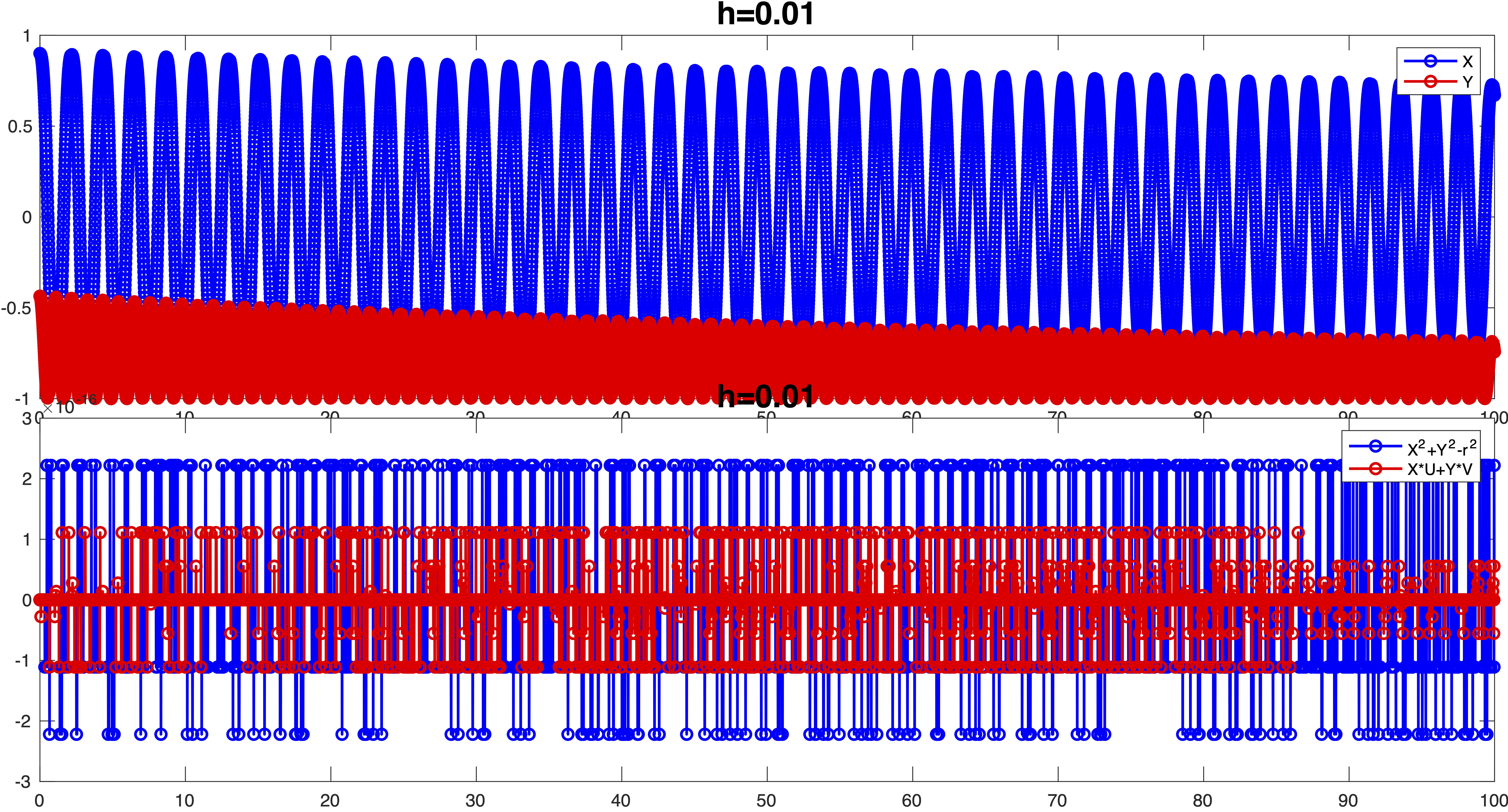
T_{\max} = 10, x(0)=0.9, u(0)=0. The remaining value y(0) = \sqrt{r^2-x(0)^2} and v(0)=-x(0)u(0)/y(0).
22.7 Runge-Kutta 4th order
\begin{aligned} K_1 &= h u_k\quad & L_1 &= h \mu\left(x_k,u_k\right)x_k \\ K_2 &= h\left(u_k+\frac{L_1}{2}\right)\quad& L_2 &= h \mu\left(x_k+\frac{K_1}{2},u_k+\frac{L_1}{2}\right)\left(x_k+\frac{K_1}{2}\right) \\ K_3 &= h\left(u_k+\frac{L_2}{2}\right)\quad & L_3 &= h\mu\left(x_k+\frac{K_2}{2},u_k+\frac{L_2}{2}\right)\left(x_k+\frac{K_2}{2}\right) \\ K_4 &= h\left(u_k+L_3\right)\quad & L_4 &= h\mu\left(x_k+K_3,u_k+L_3\right)\left(x_k+K_3\right) \end{aligned}
\begin{aligned} x_{k+1} &= x_k + \frac{K_1+2K_2+2K_3+K_4}{6} \\ u_{k+1} &= u_k + \frac{L_1+2L_2+2L_3+L_4}{6} \end{aligned}
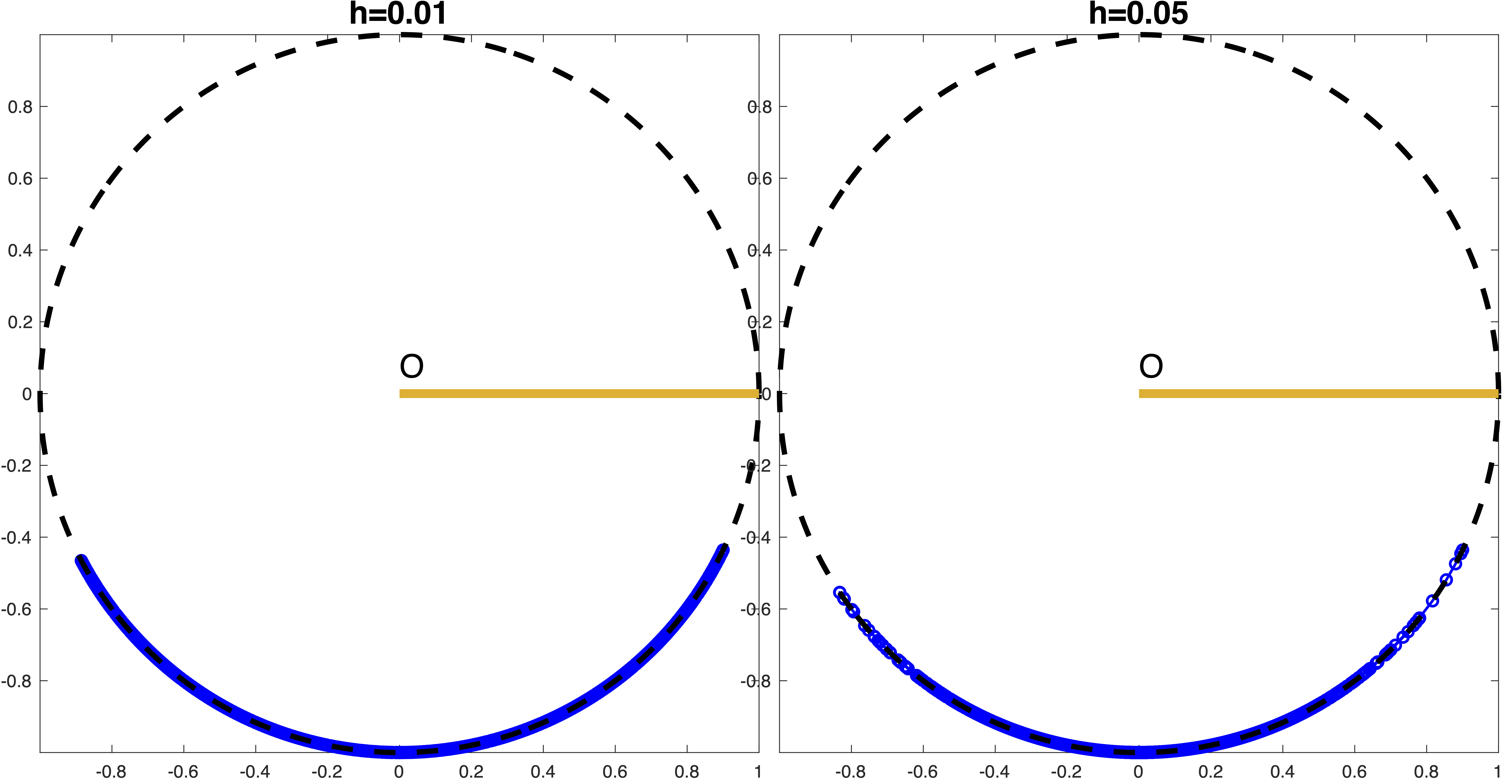
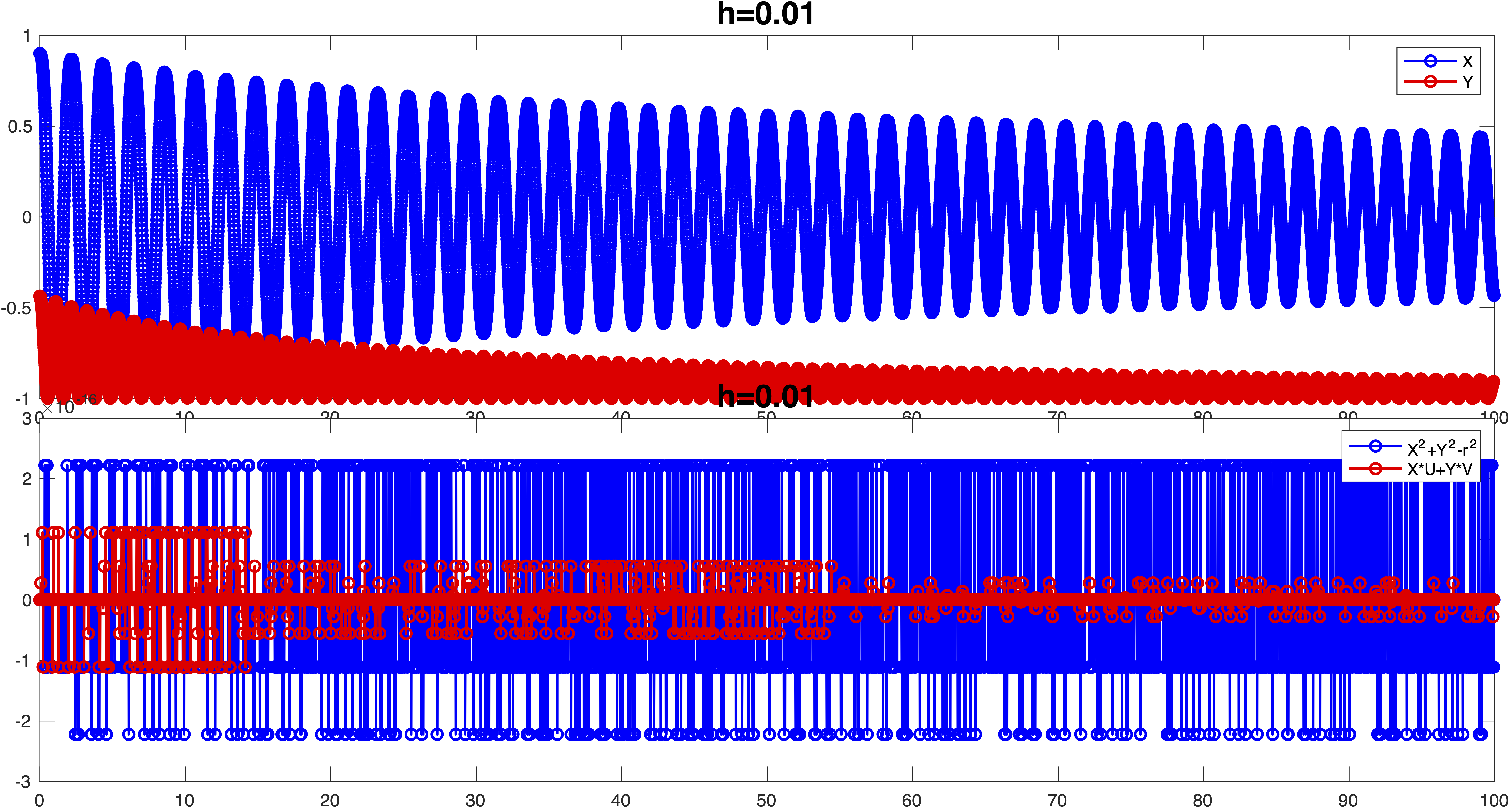
T_{\max} = 10, x(0)=0.9, u(0)=0. The remaining value y(0) = \sqrt{r^2-x(0)^2} and v(0)=-x(0)u(0)/y(0).