8 Gaussian Elimination and Echelon form

The Weierstrass canonical form is quite valuable from a theoretical standpoint. However, it can be computationally intensive since it necessitates the use of several Jordan canonical forms. In the following section, we will present a more numerically efficient algorithm for reducing a Differential Algebraic Equation (DAE) to an Ordinary Differential Equation (ODE). This method leverages the well-known Gaussian elimination technique, enhanced with differentiation to achieve the desired reduction.
8.1 Gaussian Elimination
Before diving into DAE reduction to ODE, we will revisit some fundamental concepts and definitions that are pertinent to this process.
Definition 8.1 Given a matrix
\bm{M} \in \Bbb{R}^{n \times m}
we define elementary operations as follows:
- Permutation of two rows (or columns),
- Linear combinations of rows (or columns).
These operations can also be viewed as specific forms of matrix multiplication.
Definition 8.2 A non-singular matrix
\bm{P}_{[i,j]} \in \Bbb{R}^{n \times n}
is referred to as a permutation matrix (row or column depend on the application) if it is derived from the identity matrix \bm{I} \in \Bbb{R}^{n \times n} by swapping column i with column j.
Permutation matrices exhibit several noteworthy properties:
\bm{P}_{[i,j]}^{-1} = \bm{P}_{[i,j]}^{\intercal}: This shows that \bm{P}_{[i,j]} is an orthogonal matrix.
\bm{P}_{[i,j]}^{2} = \bm{I}: This indicates that \bm{P}_{[i,j]} is an involution matrix.
\bm{P}_{[i,j]}\bm{M}: This operation exchanges row i with row j.
\bm{M} \bm{P}_{[i,j]}: This operation exchanges column i with column j.
In a similar manner, we can define matrices that perform linear combinations of rows (or columns). These matrices are classified as elementary matrices.
Definition 8.3 A matrix
\bm{F}_{[i,j]}(\alpha) \in \Bbb{R}^{n\times n}
is referred to as a row (or column) elementary matrix if it has the following structure:
\bm{F}_{[i,j]}(\alpha) = \begin{bmatrix} 1 & \dots & 0 & \dots & 0 & \dots & 0 \\ \vdots & \ddots & \vdots & & \vdots & & \vdots \\ 0 & \dots & 1 & & 0 & & 0 \\ \vdots & & \vdots & \ddots & \vdots & & \vdots \\ 0 & \dots & \alpha & \dots & 1 & \dots & 0 \\ \vdots & & \vdots & & \vdots & \ddots & \vdots \\ 0 & \dots & 0 & \dots & 0 & \dots & 1 \end{bmatrix}
where the (i,j) entry equals \alpha.
Remark 8.1. An elementary matrix \bm{F}_{[i,j]}(\alpha) \in \Bbb{R}^{n\times n} is identical to the identity matrix of dimension n in all entries except for the (i,j) position, which is set to \alpha.
Elementary matrices have several key properties:
- The operation \bm{F}_{[i,j]}(\alpha) \bm{M} adds row j multiplied by \alpha to row i.
- The operation \bm{M} \bm{F}_{[i,j]}(\alpha) adds column i multiplied by \alpha to column j.
Theorem 8.1 Given a matrix \bm{M} \in \Bbb{R}^{n \times m} with n \leq m and \text{rank}~\bm{M} = r \leq n, there exist a pair of nonsingular matrices
- \bm{L} \in \Bbb{R}^{n \times n} and
- \bm{R} \in \Bbb{R}^{m \times m}
such that
\bm{L}\bm{M}\bm{R} = \begin{bmatrix} \bm{\Lambda} & \bm{0} \\ \bm{0} & \bm{0} \end{bmatrix},
where \bm{\Lambda} \in \Bbb{R}^{r \times r} is a nonsingular diagonal matrix. The blocks of zeros have dimensions compatible with the partitioning and may be empty.
Proof. The proof follows an algorithmic approach based on sequential applications of Gaussian elimination. We define \bm{M}^{(k)}
as the matrix \bm{M} at the k-th iteration.
Note that parentheses indicate that \bm{M}^{(k)} is not the matrix \bm{M} raised to the power k. We initialize the algorithm with \bm{M}^{(1)} = \bm{M} and set k = 1.
The first step is to locate the first non-zero element within the minor
\bm{M}_{k \ldots n, k \ldots m} = \{ M_{ij}\}_{i,j=1}^{i=n,j=m}
At the first iteration, we explore all entries. We move first along the rows and then along the columns. Unless the matrix is entirely composed of zeros, we will identify a pair of indices such that M^{(k)}_{pq} \neq 0. The goal is to move this non-zero element to the (k,k) position using row and column permutations as follows:
\overline{\bm{M}}^{(k)} = \bm{P}_{[k,p]} \bm{M}^{(k)} \bm{P}_{[q,k]}.
Notice that after permutation
\overline{M}^{(k)}_{k,k} = M^{(k)}_{p,q}
thus, the non-zero element in position (p,q) of matrix \bm{M}^{(k)} is relocated to the (k,k) position of matrix \overline{\bm{M}}^{(k)}.
Next, we use this non-zero element to zero out all other entries in the k-th column and the k-th row. This can be achieved using a composition of linear combination matrices. Specifically, the matrix
\overline{\bm{L}}^{(k)} \in \Bbb{R}^{n \times n}
is designed to set all elements in the range (k+1 \ldots n, k) to zero:
\begin{aligned} \overline{\bm{L}}^{(k)} &= \bm{F}_{[k+1,k]}\left(-\frac{\overline{M}_{k+1,k}}{\overline{M}_{k,k}}\right) \cdots \bm{F}_{[n-1,k]}\left(-\frac{\overline{M}_{n-1,k}}{\overline{M}_{k,k}}\right) \bm{F}_{[n,k]}\left(-\frac{\overline{M}_{n,k}}{\overline{M}_{k,k}}\right) \\ &= \prod_{j=k+1}^{n} \bm{F}_{[j,k]}\left(-\frac{\overline{M}_{j,k}}{\overline{M}_{k,k}}\right). \end{aligned}
Similarly, we can perform the same operation along the columns. In this case, the matrix \overline{\bm{R}}^{(k)} will set all elements in the range (k, k+1 \ldots m) to zero:
\begin{aligned} \overline{\bm{R}}^{(k)} &= \bm{F}_{[k,k+1]}\left(-\frac{\overline{M}_{k,k+1}}{\overline{M}_{k,k}}\right) \cdots \bm{F}_{[k,n-1]}\left(-\frac{\overline{M}_{k,n-1}}{\overline{M}_{k,k}}\right) \bm{F}_{[k,n]}\left(-\frac{\overline{M}_{k,n}}{\overline{M}_{k,k}}\right) \\ &= \prod_{j=k+1}^{m} \bm{F}_{[k,j]}\left(-\frac{\overline{M}_{k,h}}{\overline{M}_{k,k}}\right). \end{aligned}
For notational convenience, we define the following quantities:
\begin{aligned} \bm{L}^{(k)} &= \overline{\bm{L}}^{(k)} \bm{P}_{[k,p]}, \\ \bm{R}^{(k)} &= \bm{P}_{[q,k]} \overline{\bm{R}}^{(k)}. \end{aligned}
Using both matrices \bm{L}^{(k)} \in \Bbb{R}^{n \times n} and \bm{R}^{(k)} \in \Bbb{R}^{m \times m} simultaneously, we can zero out all elements along the k-th row and the k-th column, except for the (k,k) position. The matrix \bm{M} at the next iteration is given by:
\bm{M}^{(k+1)} = \bm{L}^{(k)} \bm{M}^{(k)} \bm{R}^{(k)}.
It is now evident that by iterating this process, after exactly r iterations, the matrix \bm{M}^{(r+1)} \in \Bbb{R}^{n \times m} will have the following structure:
\bm{M}^{(r+1)} = \begin{bmatrix} \bm{\Lambda} & 0 \\ 0 & 0 \end{bmatrix}.
Moreover, the matrices \bm{L} \in \Bbb{R}^{n \times n} and \bm{R} \in \Bbb{R}^{m \times m} that achieve this structure are given by:
\begin{aligned} \bm{L} &= \bm{L}^{(r)} \bm{L}^{(r-1)} \cdots \bm{L}^{(1)}, \\ \bm{R} &= \bm{R}^{(1)} \bm{R}^{(2)} \cdots \bm{R}^{(r)}. \end{aligned}
It is important to note that both \bm{L} and \bm{R} are nonsingular since they are obtained through the product of nonsingular matrices.
To illustrate the algorithm clearly, we provide the following example.
8.2 Echelon Form
A matrix is in row echelon form if:
All nonzero rows are above rows of all zeros.
Each leading entry (first nonzero number from the left) of a row is strictly to the right of the leading entry of the row above it.
All entries in a column below a leading entry are zeros.
Example of a matrix in row echelon form:
\begin{bmatrix} \color{magenta}1 & \color{magenta}2 & \color{magenta}0 & \color{magenta}3 \\ 0 & \color{magenta}4 & \color{magenta}1 & \color{magenta}5 \\ 0 & 0 & 0 & \color{magenta}6 \\ 0 & 0 & 0 & 0 \end{bmatrix}
Another example of a matrix in row echelon form:
\begin{bmatrix} \color{magenta}1 & \color{magenta}2 & \color{magenta}3 \\ 0 & \color{magenta}4 & \color{magenta}0 \\ 0 & 0 & \color{magenta}6 \end{bmatrix}
Elementary Operations and Matrix Representation
To transform a matrix into echelon form, we use three elementary row operations, each of which corresponds to multiplying on the left by an elementary matrix:
Swapping two rows \Rightarrow Multiply by a permutation matrix.
Multiplying a row by a nonzero scalar \Rightarrow Multiply by a diagonal matrix.
Adding or subtracting a multiple of one row to another row \Rightarrow Multiply by a lower triangular matrix.
Each elementary matrix is obtained by applying the corresponding row operation to the identity matrix.
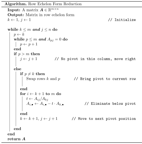
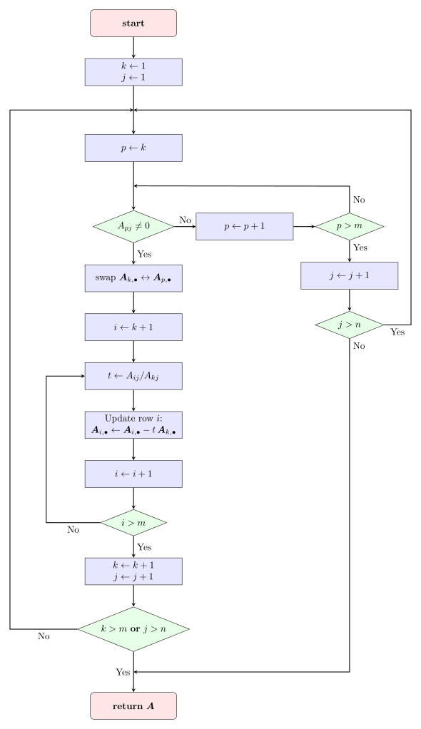
Step-by-Step Process
Step 1: Identify the Leftmost Nonzero Column (Pivot Column)
Scan the columns from left to right to find the first column that contains a nonzero entry.
The first nonzero number in that column will be our pivot.
Step 2: Ensure the Pivot is in the First Row of the Submatrix
If necessary, swap rows to move a row with a nonzero pivot to the top.
This corresponds to multiplying by a permutation matrix P.
Step 3: Zero Out All Entries Below the Pivot
For each row below the pivot row, subtract an appropriate multiple of the pivot row to make the entries below the pivot zero.
This operation is equivalent to multiplying by a lower triangular elementary matrix L.
Step 4: Normalize the Pivot (Optional but Useful)
The pivot can be scaled to 1 by dividing the row by the pivot value.
This step is equivalent to multiplying by a diagonal matrix \bm{D}.
Step 5: Move to the Next Column and Repeat
Find the next pivot column (to the right of the current pivot).
Repeat Steps 2-4 for the remaining sub-matrix.
Continue this process until all pivot positions are correctly set.
At each step, the transformation can be written as:
\bm{L}_k \bm{D}_k \bm{P}_k \cdots \bm{L}_2 \bm{D}_2 \bm{P}_2 \bm{L}_1 \bm{D}_1 \bm{P}_1 \bm{A} = \bm{U}
where \bm{U} is the echelon form of \bm{A}, and the matrices \bm{P}, \bm{D}, \bm{L} represent elementary row operations.
Example of reduction to echelon form
Given the matrix:
\bm{A} = \begin{bmatrix} 2 & 4 & 6 \\ 1 & 3 & 5 \\ 3 & 7 & 8 \end{bmatrix}
Step 1: Make the First Pivot 1
Swap row 1 and row 2 using permutation matrix \bm{P}:
\bm{P}\bm{A} = \begin{bmatrix} 1 & 3 & 5 \\ 2 & 4 & 6 \\ 3 & 7 & 8 \end{bmatrix}
Step 2: Zero Out Below the Pivot
Subtract 2 times row 1 from row 2 and 3 times row 1 from row 3 using lower triangular matrix \bm{L}_1:
\bm{L}_1 \bm{P} \bm{A} = \begin{bmatrix} 1 & 3 & 5 \\ 0 & -2 & -4 \\ 0 & -2 & -7 \end{bmatrix}
Step 3: Normalize the Second Pivot
Multiply row 2 by -\frac{1}{2} using diagonal matrix \bm{D}_1:
\bm{D}_1 \bm{L}_1 \bm{P} \bm{A} = \begin{bmatrix} 1 & 3 & 5 \\ 0 & 1 & 2 \\ 0 & -2 & -7 \end{bmatrix}
Step 4: Zero Out Below the New Pivot
Add 2 times row 2 to row 3 using lower triangular matrix \bm{L}_2:
\bm{L}_2 \bm{D}_1 \bm{L}_1 \bm{P} \bm{A} = \begin{bmatrix} \color{magenta}1 & \color{magenta}3 & \color{magenta}5 \\ 0 & \color{magenta}1 & \color{magenta}2 \\ 0 & 0 & \color{magenta}-3 \end{bmatrix}
This matrix is now in row echelon form.
Example of reduction to echelen form for a singular matrix
Consider the singular matrix:
\bm{A} = \begin{bmatrix} 2 & 4 & 6 \\ 1 & 2 & 3 \\ 3 & 6 & 9 \end{bmatrix}
Step 1: Normalize the First Pivot
Swap row 1 and row 2:
\bm{P} \bm{A} = \begin{bmatrix} 1 & 2 & 3 \\ 2 & 4 & 6 \\ 3 & 6 & 9 \end{bmatrix}
Step 2: Zero Out Below the Pivot
Subtract 2 times row 1 from row 2 and 3 times row 1 from row 3:
\bm{L}_1 \bm{P} \bm{A} = \begin{bmatrix} \color{magenta}1 & \color{magenta}2 & \color{magenta}3 \\ 0 & 0 & 0 \\ 0 & 0 & 0 \end{bmatrix}
Since the last two rows are all zeros, the rank of the matrix is 1, meaning:
- The matrix has linearly dependent rows.
- The determinant is zero, confirming singularity.
- The system \bm{A}\bm{x} = \bm{b} may have either infinitely many solutions or no solution, depending on b.
Thus, the matrix does not have an inverse.
Summary of Echelon Form Reduction Algorithm
To transform a matrix into row echelon form:
- Identify the leftmost pivot column.
- Swap rows if necessary to bring a nonzero pivot to the top \bm{P}\bm{A}.
- Zero out all entries below the pivot \bm{L}_1, \bm{L}_2, \ldots.
- Normalize pivots if needed \bm{D}_1, \bm{D}_2, \ldots.
- Move to the next pivot column and repeat.
- Continue until all pivots are set correctly.
Each row operation corresponds to multiplication by an elementary matrix, leading to the factorization:
\bm{E}_k \cdots \bm{E}_2 \bm{E}_1 \bm{A} = \bm{U}
where \bm{U} is in echelon form, and \bm{E}_i are elementary matrices.
This method is a systematic approach to solving linear systems, computing ranks, and checking singularity conditions.