19 Projection method

Another way to stabilize the constraint
\bm{\phi}(\bm{p},t)=0
and avoid the drift effect is using the projection method. The idea is to firstly reduce the index of the DAE, thus obtaining an ODE and a list of hidden constraints. Then the resulting ODE can be numerically integrated, leading to a generic intermediate solution
\widetilde{\bm{p}}(t_n).
This temporary solution is projected to the hidden constraints in order to minimize the error between the numerical integration solution and the actual system constraints, which is a nonlinear constrained least squares problem because of the norm chosen.
It should be noticed that unlike the Baumgarte’s stabilization method this technique is useful and particularly effective if you are interested in the short term behavior, since even during transients the constraint is always satisfied. Different information from the original and reduced system can be used for various projection methods. For example, we can decide to get an advantage by first projecting the ODE solution
\widetilde{\bm{p}}(t_n)
to the position constraints and than to the velocity constraints.
Example 19.1
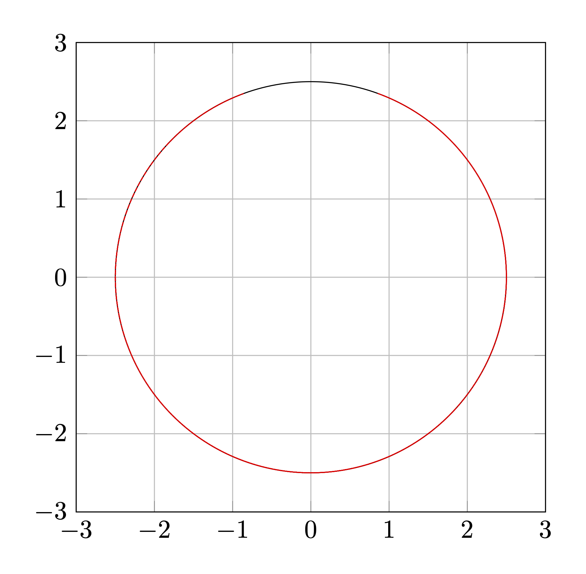
Continuing Example 19.1 we want use the Projection technique to stabilize the pendulum. The numerical scheme for integrating the reduced DAE is that in Equation 11.3. We want now to project the results of the generic ODE numerical integrator to the following hidden constraints,
\begin{aligned} \dfrac{\mathrm{d}\phi}{\mathrm{d} t} &= 2 (\bm{p}\cdot\bm{v}) = 0. \\[1em] \dfrac{\mathrm{d}^{2}\phi}{\mathrm{d} t^2} & = 2(\dot{\bm{p}}\cdot\bm{v}) + 2(\bm{p}\cdot\dot{\bm{v}}) = 2(\bm{v}\cdot\bm{v}) + 2(\bm{p}\cdot\dot{\bm{v}}) = \bm{0}. \end{aligned}
At each time step, the resulting orthogonal projection to the constraints is equal to
\begin{aligned} \text{minimize:} \quad & \dfrac{1}{2} \| \widetilde{\bm{p}} - \bm{p}\|^2 \\[1em] \text{subject to:} \quad & \bm{\phi}(\bm{p},t) = \bm{p}\cdot\bm{p} - \ell^{2} = 0 \end{aligned}
for the position coordinates projection, and
\begin{aligned} \textrm{minimize:} \quad & \dfrac{1}{2} \|\widetilde{\bm{v}} - \bm{v} \|^2 \\[1em] \text{subject to:} \quad & \frac{\mathrm{d}\bm{\phi}}{\mathrm{d}t}(\bm{p},t)=2(\bm{v}\cdot\bm{p})=0 \end{aligned}
for the velocity coordinates projection.
19.1 Projection Methods in general
Projection methods aim to leverage well-established numerical techniques to efficiently solve DAEs while ensuring consistency with their inherent constraints. The core idea is to exploit the robustness and accuracy of existing solvers for ordinary differential equations (ODEs) by transforming the problem into an ODE system with constraints and subsequently applying a projection step to maintain consistency.
Key Principles of the Projection Method
- Utilization of existing ODE Solvers:
- Many sophisticated and highly accurate solvers are available for ODEs.
- By reformulating a DAE as an ODE, one can take advantage of these mature numerical techniques.
- Many sophisticated and highly accurate solvers are available for ODEs.
- Constraint Satisfaction via Projection:
- Directly solving a transformed ODE may lead to constraint violation over time due to numerical errors, a phenomenon known as drift.
- To mitigate drift, a projection step is introduced to enforce consistency with the hidden constraints at each step or whenever the drift becomes non-negligible.
- Directly solving a transformed ODE may lead to constraint violation over time due to numerical errors, a phenomenon known as drift.
Projection Method Workflow
The projection method follows a straightforward two-step paradigm:
- ODE Step: Advance the solution using any standard numerical solver for ODEs.
- Projection Step: Adjust the computed solution by projecting it onto the manifold defined by the constraints, thereby ensuring consistency.
This approach provides a balance between computational efficiency and constraint preservation, making it an attractive method for solving DAEs.
Requirements for the Projection Method
The projection method relies on the following essential components:
- Index Reduction:
- DAEs often have a higher differential index, which makes them difficult to solve directly.
- Index reduction techniques are applied to convert the DAE into an ODE system with explicit algebraic constraints.
- DAEs often have a higher differential index, which makes them difficult to solve directly.
- Collection of Constraints and Jacobians:
- To perform projection, the constraints and their Jacobians must be determined.
- This involves symbolic computations to extract hidden constraints and their derivatives.
- To perform projection, the constraints and their Jacobians must be determined.
Thus, while the projection method simplifies numerical integration, it does not eliminate the need for symbolic preprocessing:
- Index reduction typically requires symbolic manipulations proportional to the index of the DAE.
- The projection step involves a smaller symbolic computation effort, primarily related to evaluating constraint Jacobians, whose complexity depends on the chosen projection algorithm.
19.2 Mathematical Formulation
Consider a general DAE system:
\bm{F}(\bm{x},\bm{x}^\prime,t) = \bm{0}
where \bm{x} represents the state variables, and \bm{F} defines the differential-algebraic structure.
To facilitate numerical integration, the system is transformed into an ODE system with explicit constraints using index reduction:
\begin{aligned} \bm{x}' & = \bm{G}(\bm{x},t), \quad && \textcolor{DarkGreen}{\text{[ODE]}} \\ \bm{0} & = \bm{H}(\bm{x},t), \quad && \textcolor{DarkGreen}{\text{[Invariants or hidden constraints]}} \end{aligned}
where:
- \bm{G}(\bm{x},t) defines the transformed r.h.s. of the ODE system.
- \bm{H}(\bm{x},t) represents the constraints that must be satisfied throughout the integration process.
19.3 Numerical Integration with Projection
Step 1: ODE Integration
Using an explicit numerical scheme, such as the explicit Euler method, we compute a preliminary update:
\widetilde{\bm{x}}_{k+1} = \bm{x}_{k} + \Delta t\,\bm{G}(\bm{x}_k,t_k)
where \widetilde{\bm{x}}_{k+1} is the intermediate solution, which may not satisfy the constraints due to numerical errors.
Step 2: Projection onto the Constraint Manifold
To restore consistency, the next step is to compute the corrected state \bm{x}_{k+1} by solving the constrained optimization problem:
\begin{aligned} \textrm{minimize} \quad & f(\textcolor{red}{\bm{z}}) = \frac{1}{2} \|\textcolor{red}{\bm{z}} - \widetilde{\bm{x}}_{k+1} \|^2 \\ \textrm{subject to the constraint:}\quad & \bm{H}(\textcolor{red}{\bm{z}}, t_{k+1}) = \bm{0}. \end{aligned}
then set \bm{x}_{k+1}=\textcolor{red}{\bm{z}}.
This optimization step ensures that \bm{x}_{k+1} remains on the constraint manifold, effectively eliminating the drift introduced by numerical integration.
19.4 Generic Minimization Problem with Constraints
In many numerical applications, we encounter the problem of minimizing a function while satisfying a set of constraints. The general form of such a constrained optimization problem is:
\text{minimize} \quad f(\textcolor{red}{\bm{z}}) \quad \text{subject to} \quad \bm{h}(\textcolor{red}{\bm{z}}) = \bm{0}
where:
- f(\bm{z}) is the objective function to be minimized.
- \bm{h}(\bm{z}) represents the set of constraints that must be satisfied.
Here is shown a sketch in matlab for the solution of constrained minimization problem using function fmincon:
% Dimensione di z
n = ...;

% objective function f(z)
objective = @(z) ...;

% constraint h(z)
nonlcon = @(z) ...;

% Initial point
z0 = xtilde;

% Solve using fmincon
options = optimoptions(  'fmincon', ...
  'Display',             'iter',  ...
  'Algorithm',           'sqp',   ...
  'MaxIterations',       100,     ...
  'OptimalityTolerance', 1e-8     ...
);

z_sol = fmincon( objective, z0, ...
                 [], [], [], [], [], [], ...
                 nonlcon, options);
Solution Using Lagrange Multipliers
To find the solution, we introduce the Lagrangian function:
\mathcal{L}(\textcolor{red}{\bm{z}},\textcolor{blue}{\bm{\lambda}}) = f(\textcolor{red}{\bm{z}}) - \textcolor{blue}{\bm{\lambda}} \cdot \bm{h}(\textcolor{red}{\bm{z}})
where:
- \textcolor{blue}{\bm{\lambda}} is the vector of Lagrange multipliers, which enforces the constraints.
The necessary conditions for a solution (also called the Karush-Kuhn-Tucker conditions) correspond to the stationary points of the Lagrangian:
\left\{ \begin{aligned} \dfrac{\partial\mathcal{L}(\bm{z},\bm{\lambda})}{\partial\bm{z}} &= \bm{0}, \\[1em] \dfrac{\partial\mathcal{L}(\bm{z},\bm{\lambda})}{\partial\bm{\lambda}} &= \bm{0}. \end{aligned} \right.
Expanding these derivatives explicitly:
\left\{ \begin{aligned} \nabla f(\bm{z}) - \bm{h}_{\bm{z}}(\bm{z})^T \bm{\lambda} & = \bm{0}, \\[0.5em] \bm{h}(\bm{z}) & = \bm{0}. \end{aligned} \right.
where \bm{h}_{\bm{z}} is the Jacobian matrix of the constraints:
\bm{h}_{\bm{z}} = \frac{\partial \bm{h}(\bm{z})}{\partial \bm{z}}.
This system of nonlinear equations must be solved to find the optimal solution (\bm{z}, \bm{\lambda}).
Linearization of the Minimization Problem
Since the nonlinear system above is often difficult to solve directly, we employ a linearization technique around a current estimate \bm{z}. This leads to an iterative solution approach.
By performing a first-order Taylor expansion of the necessary conditions with respect to \bm{z}, we obtain:
\left\{ \begin{aligned} \nabla f(\bm{z}) + \textcolor{red}{\nabla^2 f(\bm{z}) \delta \bm{z}} - \bm{h}_{\bm{z}}(\bm{z})^T \bm{\lambda} & = \textcolor{blue}{\mathcal{O}(\|\delta \bm{z}\|^2)}, \\[1em] \bm{h}(\bm{z})+ \textcolor{red}{\bm{h}_{\bm{z}}(\bm{z}) \delta \bm{z}} & = \textcolor{blue}{\mathcal{O}(\|\delta \bm{\lambda}\|^2)}. \end{aligned} \right.
Ignoring the higher-order terms \mathcal{O}(\|\delta \bm{z}\|^2), we derive an iterative Newton-like method for solving the optimization problem.
Iterative Algorithm for the Constrained Minimization Problem
Initialize with an initial guess \bm{z}_0 = \widetilde{\bm{x}}_{k+1}.
Update the solution iteratively:
\bm{z}_{\ell+1} = \bm{z}_{\ell} + \delta\bm{z}, \quad \ell = 0,1,\ldots \quad \text{(until convergence)}.
Solve for the update \delta \bm{z} by solving the following linear system:
\begin{pmatrix} \nabla^2 f(\bm{z}_{\ell}) & -\bm{h}_{\bm{z}}(\bm{z}_{\ell})^T \\[1em] -\bm{h}_{\bm{z}}(\bm{z}_{\ell}) & \bm{0} \end{pmatrix} %%% \begin{pmatrix} \delta\bm{z}\\[1em] \textcolor{blue}{\bm{\lambda}} \end{pmatrix} = \begin{pmatrix} -\nabla f(\bm{z}_{\ell})\\[1em] \bm{h}(\bm{z}_{\ell}) \end{pmatrix}
This system provides the correction \delta\bm{z} for the next iteration step.
Special Case: Quadratic Objective Function
A particularly important case is when the objective function is quadratic, given by:
f(\bm{z}) = \frac{1}{2} \|\bm{z} - \widetilde{\bm{x}}_{k+1}\|^2.
For this choice of f(\bm{z}), the gradient and Hessian simplify to:
\nabla f(\bm{z}) = \bm{z} - \widetilde{\bm{x}}_{k+1}, \qquad \nabla^2 f(\bm{z}) = \bm{I}.
Thus, the linear system simplifies to:
\begin{pmatrix} \bm{I} & -\bm{h}_{\bm{z}}(\bm{z}_{\ell})^T \\[1em] -\bm{h}_{\bm{z}}(\bm{z}_{\ell}) & \bm{0} \end{pmatrix} %%% \begin{pmatrix} \delta\bm{z}\\[1em] \textcolor{blue}{\bm{\lambda}} \end{pmatrix} = \begin{pmatrix} \widetilde{\bm{x}}_{k+1} - \bm{z}_{\ell}\\[1em] \bm{h}(\bm{z}_{\ell}) \end{pmatrix}
This case is particularly useful in applications like projection methods for constrained dynamics, where \widetilde{\bm{x}}_{k+1} represents an unconstrained update that needs to be corrected to satisfy the constraints \bm{h}(\bm{z}) = \bm{0}.
A sketch in matlab for the projection solution is shown here:
n      = ...; % dimension of the problem
m      = ...; % number of constraints
xt     = ...; % point to be projected
H_fun  = @(z) ...; % The constraints m x 1 matrix
Hz_fun = @(z) ...; % Jacobian of the constraints m x n matrix
z      = xt; % initial point
for k=1:max_iter
  Hz  = Hz_fun( z );
  H   = H_fun( z );
  M   = [ eye(n), Hz.' ; Hz, zeros(n,n) ];
  b   = [ xt - z; H ];
  sol = M \ b;
  dz  = sol(1:n);
  if norm(dz,inf) < tolerance
    break;
  end
  z = z+dz;
end