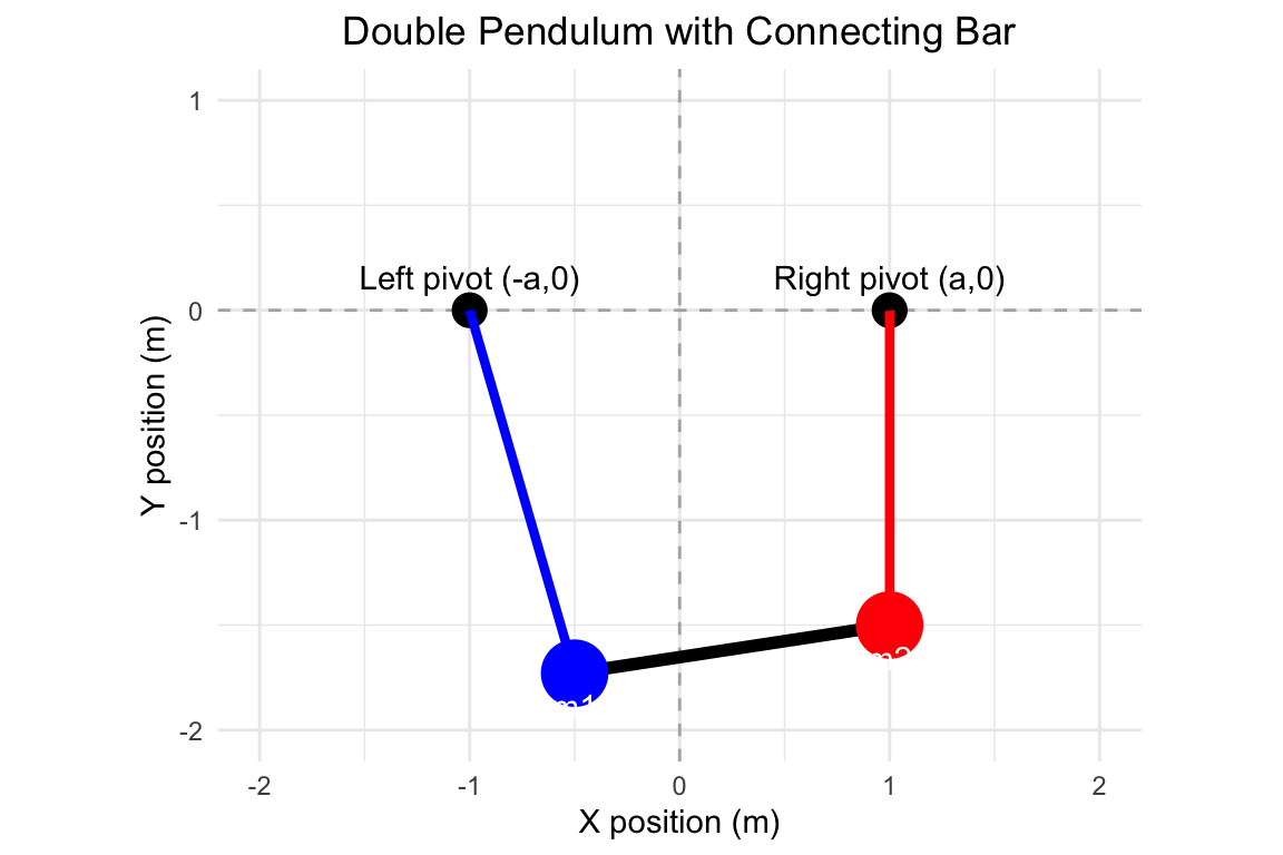
31  Example 9

Author

Affiliations

Enrico Bertolazzi

University of Trento, Department of Industrial Engineering

A constrained mechanical system consisting of two rigid pendulums connected by a fixed-length bar. In details

1. Left Pendulum Assembly:
   • Pivot: Fixed at point (-a, 0)
   • Mass m_1 located at (x_1,y_1)
   • Constraint: Rigid rod maintains length \ell_1^2 = (x_1+a)^2 + y_1^2
2. Right Pendulum Assembly:
   • Pivot: Fixed at point (a, 0)
   • Mass m_2 located at (x_2,y_2)
   • Length \ell_2^2 = (x_2-a)^2 + y_2^2 fixed
3. Coupling Mechanism:
   • Connecting bar: Rigid link between m_1 and m_2
   • Constraint: Rigid rod maintains length \ell_3^2 = (x_1-x_2)^2 + (y_1-y_2)^2

31.1 Double Pendulum System with Connecting Bar

DAE System Derivation

Now the Differential-Algebraic Equations (DAE) for the double pendulum system with a connecting bar is derived.

We employ Cartesian coordinates with the following state variables:

• Position states:
  • (x_1,y_1): Coordinates of left mass m_1​
  • (x_2,y_2): Coordinates of right mass m_2 ​
• Velocity states:
  • (u_1,v_1): Velocity components of m_1​
  • (u_2,v_2): Velocity components of m_2
• Constraint forces:
  • \lambda_1: Multiplier for left pendulum constraint
  • \lambda_2: Multiplier for right pendulum constraint
  • \lambda_3: Multiplier for connecting bar constraint

Applying Lagrange multiplier method with constraints yields:

Equations of Motion

For mass m_1

\left\{ \begin{aligned} m_1u'_1 &= -\lambda_1(x_1 + a) - \lambda_3(x_1 - x_2) \\ m_1v'_1 &= -\lambda_1y_1 - \lambda_3(y_1 - y_2) - m_1g \end{aligned} \right.

For mass m_2

\left\{ \begin{aligned} m_2u'_2 &= -\lambda_2(x_2 - a) + \lambda_3(x_1 - x_2) \\ m_2v'_2 &= -\lambda_2y_2 + \lambda_3(y_1 - y_2) - m_2g \end{aligned} \right.

Constraint Equations (Algebraic)

\left\{ \begin{aligned} (x_1 + a)^2 + y_1^2 &= \ell_1^2 \\ (x_2 - a)^2 + y_2^2 &= \ell_2^2 \\ (x_1 - x_2)^2 + (y_1 - y_2)^2 &= \ell_3^2 \end{aligned} \right.

Complete DAE Structure

Introducing

\delta x = x_1-x_2, \quad \delta y = y_1-y_2, \quad \delta u = u_1-u_2, \quad \delta v = v_1-v_2,

the complete DAE system is:

Differential Part

\left\{ \begin{aligned} x'_1 &= u_1 \\ y'_1 &= v_1 \\ x'_2 &= u_2 \\ y'_2 &= v_2 \\ m_1 u'_1 &= -(x_1+a)\lambda_1 -\delta x\lambda_3 \\[0.5em] m_1 v'_1 &= -y_1\lambda_1 -\delta y\lambda_3-m_1 g \\[0.5em] m_2 u'_2 &= -(x_2-a)\lambda_2 + \delta x\lambda_3 \\[0.5em] m_2 v'_2 &= -y_2\lambda_2 + \delta y\lambda_3-m_2 g \end{aligned} \right.

Algebraic Part

\left\{ \begin{aligned} (x_1 + a)^2 + y_1^2 - \ell_1^2 & = 0, \quad\text{(Constraint 1)}\\[0.5em] (x_2 - a)^2 + y_2^2 - \ell_2^2 & = 0, \quad\text{(Constraint 2)} \\[0.5em] \delta x^2 + \delta y^2 - \ell_3^2 & = 0, \quad\text{(Constraint 3)} \end{aligned} \right.

Semi-Explicit Formulation

Decomposes previous DAE into differential (blue) and algebraic (red) components:

\left\{ \color{blue} \begin{aligned} x'_1 &= u_1 \\ y'_1 &= v_1 \\ x'_2 &= u_2 \\ y'_2 &= v_2 \\ u'_1 &= \dfrac{-(x_1+a)\lambda_1 -\delta x\lambda_3}{m_1} \\[0.5em] v'_1 &= \dfrac{-y_1\lambda_1 - \delta y\lambda_3}{m_1}-g \\[0.5em] u'_2 &= \dfrac{-(x_2-a)\lambda_2 + \delta x\lambda_3}{m_2} \\[0.5em] v'_2 &= \dfrac{-y_2\lambda_2 + \delta y\lambda_3}{m_2}-g \end{aligned} \right. \quad \bigoplus \quad \left\{ \color{DarkRed} \begin{aligned} (x_1 + a)^2 + y_1^2 - \ell_1^2 & = 0, \quad\text{(Constraint 1)}\\[0.5em] (x_2 - a)^2 + y_2^2 - \ell_2^2 & = 0, \quad\text{(Constraint 2)} \\[0.5em] \delta x^2 + \delta y^2 - \ell_3^2 & = 0, \quad\text{(Constraint 3)} \end{aligned} \right.

For this DAE we have:

• Differential variables: x_1, y_1, x_2, y_2, u_1, v_1, u_2, v_2.
• Algebraic variables: \lambda_1, \lambda_2, \lambda_3.

no dummy variable are required.

Index Reduction Procedure

We attempt to solve for \lambda_1, \lambda_2 and \lambda_3 but the system is not yet solvable explicitly. We proceed by differentiating.

Step 1: Differentiate algebraic constraints

Now we must derivate the constraints in order to reduce the index. Here we want to differentiate only the algebraic equation that can reduce the index and do not introduce new differential equation. Here we want to avoid to introduce derivatove of the algebraic variable unless is strictly necessary.

We construct a dependency table to identify which constraints to differentiate:

\begin{array}{c|ccc} & \lambda_1 & \lambda_2 & \lambda_3 \\[1em] \hline \\[0.1em] \text{(Constraint 1)} & 0 & 0 & 0 \\[1em] \text{(Constraint 2)} & 0 & 0 & 0 \\[1em] \text{(Constraint 3)} & 0 & 0 & 0 \end{array}

a 0 means the the function do not depend on the variable on the column. A 1 means dependence. All constraint are candidate for differentiation as it doesn’t introduce new algebraic variables. Differentiate thus the constraints and substitute known variable in differential form using the ODE part

\begin{aligned} \text{(Constraint 1)}' &= 2(x_1 + a)x'_1+2y_1 y'_1 = 2(x_1 + a)u_1+2y_1 v_1 \\ \text{(Constraint 2)}' &= 2(x_2 - a)x'_2+2y_2 y'_2 = 2(x_2 - a)u_2+2y_2 v_2\\ \text{(Constraint 3)}' &= 2\delta x \delta x' +2 \delta y \delta y' = 2 \delta x \delta u +2 \delta y \delta v \end{aligned}

so that the DAE become:

\left\{ \color{blue} \begin{aligned} x'_1 &= u_1 \\ y'_1 &= v_1 \\ x'_2 &= u_2 \\ y'_2 &= v_2 \\ u'_1 &= \dfrac{-(x_1+a)\lambda_1 -\delta x\lambda_3}{m_1} \\[0.5em] v'_1 &= \dfrac{-y_1\lambda_1 - \delta y\lambda_3}{m_1}-g \\[0.5em] u'_2 &= \dfrac{-(x_2-a)\lambda_2 + \delta x\lambda_3}{m_2} \\[0.5em] v'_2 &= \dfrac{-y_2\lambda_2 +\delta y\lambda_3}{m_2}-g \end{aligned} \right. \quad \bigoplus \quad \left\{ \color{DarkRed} \begin{aligned} 2(x_1 + a)u_1+2y_1 v_1& = 0,\quad\text{(Constraint 1)}'\\[0.5em] 2(x_2 - a)u_2+2y_2 v_2& = 0,\quad\text{(Constraint 2)}'\\[0.5em] 2 \delta x \delta u+2 \delta y \delta v& = 0,\quad\text{(Constraint 3)}'\\[2em] \color{DarkGreen} (x_1 + a)^2 + y_1^2 - \ell_1^2 & \color{DarkGreen} = 0, \quad\text{(Constraint 1)}\\[0.5em] \color{DarkGreen}(x_2 - a)^2 + y_2^2 - \ell_2^2 & \color{DarkGreen} = 0, \quad\text{(Constraint 2)} \\[0.5em] \color{DarkGreen} \delta x^2 + \delta y^2 - \ell_3^2 & \color{DarkGreen} = 0, \quad\text{(Constraint 3)} \end{aligned} \right.

The red algebraic equations are the new algebraic equation after the derivation. The green algebraic equation is the hidden constraints that is removed from the DAE system but that is satisfied by choosing the right initial conditions.

The red part cannot determine the algebraic variable and must be differentiated again.

Step 2: Differentiate (again) the algebraic constraints

To find the right candidate(s) here we write a table of the dependencies \begin{array}{c|ccc} & \lambda_1 & \lambda_2 & \lambda_3 \\[1em] \hline \\[0.1em] \text{(Constraint 1)}' & 0 & 0 & 0 \\[1em] \text{(Constraint 2)}' & 0 & 0 & 0 \\[1em] \text{(Constraint 3)}' & 0 & 0 & 0 \end{array}

Again all the constraints can be differentiated

\begin{aligned} \text{(Constraint 1)}'' &= 2x'_1u_1+2y'_1 v_1+ 2(x_1 + a)u'_1+2y_1 v'_1\\ &= 2(u_1^2+v_1^2)+ 2(x_1 + a)u'_1+2y_1 v'_1\\ \text{(Constraint 2)}'' &= 2x'_2u_2+2y'_2v_2+ 2(x_2 - a)u'_2+2y_2 v'_2\\ &= 2(u_2^2+v_2^2)+ 2(x_2 - a)u'_2+2y_2 v'_2\\ \text{(Constraint 3)}'' &= 2\delta x'\delta u + 2\delta x\delta u'+ 2\delta y'\delta v + 2\delta y\delta v' \\ &= 2(\delta u^2+\delta v^2) + 2\delta x \delta u' +2 \delta y \delta v' \end{aligned}

the substitution of the derivative make the constraint complex. Thus, dummy variable are introduced to reduce complexity:

\begin{aligned} \text{(Constraint 1)}'' &= 2(u_1^2+v_1^2)+ 2(x_1 + a)u_{1,\text{dot}}+2y_1 v_{1,\text{dot}}\\ \text{(Constraint 2)}'' &= 2(u_2^2+v_2^2)+ 2(x_2 - a)u_{2,\text{dot}}+2y_2 v_{2,\text{dot}}\\ \text{(Constraint 3)}'' &= 2(\delta u^2+\delta v^2) + 2\delta x (u_{1,\text{dot}}-u_{2,\text{dot}}) + 2 \delta y (v_{1,\text{dot}}-v_{2,\text{dot}}) \end{aligned}

and the DAE, introducing

\delta u_{\text{dot}} = u_{1,\text{dot}}-u_{2,\text{dot}}, \qquad \delta v_{\text{dot}} = v_{1,\text{dot}}-v_{2,\text{dot}}

become:

\left\{ \color{blue} \begin{aligned} x'_1 &= u_1 \\ y'_1 &= v_1 \\ x'_2 &= u_2 \\ y'_2 &= v_2 \\ u'_1 &= u_{1,\text{dot}} \\ v'_1 &= v_{1,\text{dot}} \\ u'_2 &= u_{2,\text{dot}} \\ v'_2 &= v_{2,\text{dot}} \end{aligned} \right. \quad \bigoplus \quad \left\{ \color{DarkRed} \begin{aligned} 2(u_1^2+v_1^2)+ 2(x_1 + a)u_{1,\text{dot}}+2y_1 v_{1,\text{dot}} & = 0,\quad\text{(Constraint 1)}''\\[0.5em] 2(u_2^2+v_2^2)+ 2(x_2 - a)u_{2,\text{dot}}+2y_2 v_{2,\text{dot}} & = 0,\quad\text{(Constraint 2)}''\\[0.5em] 2(\delta u^2+\delta v^2) + 2\delta x \delta u_{\text{dot}} + 2 \delta y \delta v_{\text{dot}} & = 0,\quad\text{(Constraint 3)}''\\[0.5em] m_1 u_{1,\text{dot}} +(x_1+a)\lambda_1+\delta x\lambda_3 &=0,\quad\text{(Constraint 4)} \\[0.5em] m_1 v_{1,\text{dot}}+y_1\lambda_1+\delta y\lambda_3+m_1 g &=0,\quad\text{(Constraint 5)} \\[0.5em] m_2 u_{2,\text{dot}}+(x_2-a)\lambda_2-\delta x\lambda_3 &=0,\quad\text{(Constraint 6)} \\[0.5em] m_2 v_{2,\text{dot}}+y_2\lambda_2-\delta y\lambda_3+m_2g &=0,\quad\text{(Constraint 7)} \\[2em] \color{DarkGreen} 2(x_1 + a)u_1+2y_1 v_1 & \color{DarkGreen} = 0,\quad\text{(Constraint 1)}'\\[0.5em] \color{DarkGreen} 2(x_2 - a)u_2+2y_2 v_2 & \color{DarkGreen} = 0,\quad\text{(Constraint 2)}'\\[0.5em] \color{DarkGreen} 2 \delta x \delta u+2 \delta y \delta v & \color{DarkGreen} = 0,\quad\text{(Constraint 3)}'\\[2em] \color{DarkGreen} (x_1 + a)^2 + y_1^2 - \ell_1^2 & \color{DarkGreen} = 0, \quad\text{(Constraint 1)}\\[0.5em] \color{DarkGreen}(x_2 - a)^2 + y_2^2 - \ell_2^2 & \color{DarkGreen} = 0, \quad\text{(Constraint 2)} \\[0.5em] \color{DarkGreen} \delta x^2 + \delta y^2 - \ell_3^2 & \color{DarkGreen} = 0, \quad\text{(Constraint 3)} \end{aligned} \right.

The red algebraic equations are the new algebraic equation after the derivation. Notice the four new algebraic constraints added from the introduction of dummy variables. The green algebraic equation is the hidden constraints that is removed from the DAE system but that is satisfied by choosing the right initial conditions.

Step 3: Differentiate the algebraic constraints?

To find the right candidate(s) here we write a table of the dependencies. Notice that now the table is larger due to the introduction of new dummy variables and four new constraints

\begin{array}{c|ccccccc} & \lambda_1 & \lambda_2 & \lambda_3 & u_{1,\text{dot}} & v_{1,\text{dot}} & u_{2,\text{dot}} & v_{2,\text{dot}} \\[1em] \hline \\[0.1em] \text{(Constraint 1)}'' & 0 & 0 & 0 & 1 & 1 & 0 & 0 \\[1em] \text{(Constraint 2)}'' & 0 & 0 & 0 & 0 & 0 & 1 & 1 \\[1em] \text{(Constraint 3)}'' & 0 & 0 & 0 & 1 & 1 & 1 & 1 \\[1em] \text{(Constraint 4)} & 1 & 0 & 1 & 1 & 0 & 0 & 0 \\[1em] \text{(Constraint 5)} & 1 & 0 & 1 & 0 & 1 & 0 & 0 \\[1em] \text{(Constraint 6)} & 0 & 1 & 1 & 0 & 0 & 1 & 0 \\[1em] \text{(Constraint 7)} & 0 & 1 & 1 & 0 & 0 & 0 & 1 \end{array}

Again all the constraints cannot be differentiated. At this point we must check if the jacobian of the constraints is non-singular. If is non-singular formally we can solve for \lambda_1, \lambda_2, \lambda_3, u_{1,\text{dot}}, v_{1,\text{dot}}, u_{2,\text{dot}} and v_{2,\text{dot}} and the DAE is of index-1 and we can stop index reduction. To check if jacobian is singular before to try LU decomposion we analize the nonzero structure of the jacobian \bm{S}

\bm{S} = \begin{pmatrix} \cdot & \cdot & \cdot & 1 & 1 & \cdot & \cdot \\ \cdot & \cdot & \cdot & \cdot & \cdot & 1 & 1 \\ \cdot & \cdot & \cdot & 1 & 1 & 1 & 1 \\ 1 & \cdot & 1 & 1 & \cdot & \cdot & \cdot \\ 1 & \cdot & 1 & \cdot & 1 & \cdot & \cdot \\ \cdot & 1 & 1 & \cdot & \cdot & 1 & \cdot \\ \cdot & 1 & 1 & \cdot & \cdot & \cdot & 1 \end{pmatrix}

In this form is difficult to understand if a matrix with nonzero at the 1 position can be non-singular.

We use sprank of MATLAB to check if the matrix can be non singular.

sparsity_pattern = [
  0 0 0 1 1 0 0;  % Constraint 1''
  0 0 0 0 0 1 1;  % Constraint 2''
  0 0 0 1 1 1 1;  % Constraint 3''
  1 0 1 1 0 0 0;  % Constraint 4
  1 0 1 0 1 0 0;  % Constraint 5
  0 1 1 0 0 1 0;  % Constraint 6
  0 1 1 0 0 0 1]; % Constraint 7

fprintf('Estimated rank = %d\n', sprank(sparsity_pattern) )

> Estimated rank = 7

The estimated rank is 7 so that matrix is structurally non-simgular.

To better understand how it work consider the Dulmage-Mendelsohn decomposition that find rows and columns permutation for maximum mathcing

[p,q,r,s,cc,rr] = dmperm(sparsity_pattern)

sparsity_pattern(p,q)

ans =

     1     0     1     1     0     0     0
     0     1     1     0     0     1     0
     1     0     1     0     1     0     0
     0     0     0     1     1     0     0
     0     0     0     1     1     1     1
     0     0     0     0     0     1     1
     0     1     1     0     0     0     1

you can see that the diagonal is all 1 thus a matrix with element non zero only on the diagonal is surely non singular. In practice

• do Dulmage-Mendelsohn decomposition
• Apply rows and columns permutation
• If the diadonal is non zeros (all 1) the matrix is structurally non singular.

Here, here we can do a step more because the system is linear. Let

\bm{X} = \begin{pmatrix} x_1 \\ y_1 \\ x_2 \\ y_2 \\ u_1 \\ v_1 \\ u_2 \\ v_2 \end{pmatrix}, \quad \bm{Z} = \begin{pmatrix} \lambda_1 \\ \lambda_2 \\ \lambda_3 \\ u_{1,\text{dot}} \\ v_{1,\text{dot}} \\ u_{2,\text{dot}} \\ v_{2,\text{dot}} \end{pmatrix}

then constraint become

\bm{A}(\bm{X},t)\bm{Z} = \bm{b}(\bm{X},t)

where \bm{A}(\bm{X},t) = \begin{pmatrix} 0 & 0 & 0 & x_1+a & y_1 & 0 & 0 \\ 0 & 0 & 0 & 0 & 0 & x_2-a & y_2 \\ 0 & 0 & 0 & \delta x & \delta y & -\delta x & -\delta y \\ x_1+a & 0 & \delta x & m_1 & 0 & 0 & 0 \\ y_1 & 0 & \delta y & 0 & m_1 & 0 & 0 \\ 0 & x_2-a & -\delta x & 0 & 0 & m_2 & 0 \\ 0 & y_2 & -\delta y & 0 & 0 & 0 & m_2 \end{pmatrix}

and

\bm{b}(\bm{X},t) = -\begin{pmatrix} u_1^2+v_1^2 \\ u_2^2+v_2^2 \\ \delta u^2+\delta v^2 \\ 0\\ m_1 g \\ 0 \\ m_2 g \\ \end{pmatrix}

and the DAE become

\left\{ \color{blue} \begin{aligned} x'_1 &= u_1 \\ y'_1 &= v_1 \\ x'_2 &= u_2 \\ y'_2 &= v_2 \\ u'_1 &= u_{1,\text{dot}} \\ v'_1 &= v_{1,\text{dot}} \\ u'_2 &= u_{2,\text{dot}} \\ v'_2 &= v_{2,\text{dot}} \\ \bm{A}(\bm{X},t) \bm{Z} & = \bm{b}(\bm{X},t) \end{aligned} \right. \quad \bigoplus \quad \left\{ \color{DarkGreen} \begin{aligned} 2(x_1 + a)u_1+2y_1 v_1 & = 0,\quad\text{(Constraint 1)}'\\[0.5em] 2(x_2 - a)u_2+2y_2 v_2 & = 0,\quad\text{(Constraint 2)}'\\[0.5em] 2 \delta x \delta u+2 \delta y \delta v & = 0,\quad\text{(Constraint 3)}'\\[2em] (x_1 + a)^2 + y_1^2 - \ell_1^2 & = 0, \quad\text{(Constraint 1)}\\[0.5em] (x_2 - a)^2 + y_2^2 - \ell_2^2 & = 0, \quad\text{(Constraint 2)} \\[0.5em] \delta x^2 + \delta y^2 - \ell_3^2 & = 0, \quad\text{(Constraint 3)} \end{aligned} \right.

where the green part are the hidden constraints that are satisfied by choosing the correct initial conditions.

Completion will follow the conclusion of the second part of the assignment.