18 Baumgarte’s stabilization
18.1 Differential-Algebraic Equations (DAEs) in Mechanics
This document offers an in-depth exploration of how Differential-Algebraic Equations (DAEs) are formulated and numerically solved, particularly within the context of mechanical systems. It emphasizes systems that involve constraints, which commonly appear in areas like multibody dynamics, robotics, and structural mechanics.
Notation and Setup
Consider a mechanical system with the following quantities:
- Generalized (position) coordinates: \bm{p} \in \Bbb{R}^n, representing the configuration of the system.
- Kinetic energy: T(\bm{p}, \bm{p}^{\prime}, t), where \bm{p}^{\prime} is the time derivative of \bm{p}.
- Potential energy: V(\bm{p}, t).
- External generalized forces: \bm{Q}_{ex}(\bm{p}, t) \in \Bbb{R}^n.
- Constraint equations: \bm{\Phi}(\bm{p}, t) \in \Bbb{R}^m, which enforce m constraints on the system.
- Lagrangian:
L(\bm{p}, \bm{p}^{\prime}, t) = T(\bm{p}, \bm{p}^{\prime}, t) - V(\bm{p}, t).
The equations of motion are derived from Lagrange’s equations with constraints:
\frac{\mathrm{d}}{\mathrm{d}t} \left( \frac{\partial L}{\partial \bm{p}^{\prime}} \right) - \frac{\partial L}{\partial \bm{p}} + \left( \frac{\partial \bm{\Phi}(\bm{p}, t)}{\partial \bm{p}} \right)^T \bm{\lambda} = \bm{Q}_{ex}(\bm{p}, \bm{p}^{\prime},t),
where \bm{\lambda} \in \Bbb{R}^m are the Lagrange multipliers enforcing the constraints.
Reformulating as a DAE
Kinetic Energy and Mass Matrix
The kinetic energy is often expressed in terms of the mass matrix \bm{M}(\bm{p},\bm{p}',t):
T(\bm{p}, \bm{p}^{\prime}, t) = \frac{1}{2} (\bm{p}^{\prime})^T \bm{M}(\bm{p},\bm{p}',t) \bm{p}^{\prime}.
Substituting this into the equations of motion yields:
\bm{M}(\bm{p},\bm{p}^{\prime},t) \bm{p}^{\prime\prime} + \left( \frac{\partial \bm{\Phi}}{\partial \bm{p}} \right)^T \bm{\lambda} = \bm{Q}(\bm{p}, \bm{p}^{\prime}, t),
where \bm{Q}(\bm{p}, \bm{p}^{\prime}, t) includes external forces, potential energy gradients, and inertial terms.
Constraint Equations
The constraints \bm{\Phi}(\bm{p}, t) = 0 must be satisfied at all times. Combining these with the equations of motion, we obtain the full DAE system:
\left\{ \begin{aligned} \bm{M}(\bm{p},\bm{p}^\prime t) \bm{p}^{\prime\prime} + \bm{\Phi}_{\bm{p}}(\bm{p}, t)^T \bm{\lambda} &= \bm{Q}(\bm{p}, \bm{p}^{\prime}, t), \\[0.5em] \bm{\Phi}(\bm{p}, t) &= \bm{0}. \end{aligned} \right.
This system has n + m equations and n + m unknowns (\bm{p}^{\prime\prime} and \bm{\lambda}), making it well-posed.
18.2 Numerical Solution of DAEs
Solving DAEs requires specialized numerical methods due to the presence of algebraic constraints. Below, we outline a common approach based on time discretization and constraint differentiation.
Time Discretization
A simple numerical scheme can be derived using a Taylor expansion in time:
\begin{aligned} \bm{p}^{\prime}(t+\Delta t) &= \bm{p}^{\prime}(t) + \bm{p}^{\prime\prime}(t) \Delta t + \mathcal{O}(\Delta t^2), \\[1em] \bm{p}(t+\Delta t) &= \bm{p}(t) + \bm{p}^{\prime}(t) \Delta t + \frac{1}{2} \bm{p}^{\prime\prime}(t) \Delta t^2 + \mathcal{O}(\Delta t^3). \end{aligned}
Neglecting higher-order terms, the updates for position and velocity become:
\begin{aligned} \bm{p}^{\prime}_{k+1} &= \bm{p}^{\prime}_k + {\color{red} \bm{p}^{\prime\prime}_k} \Delta t, \\[1em] \bm{p}_{k+1} &= \bm{p}_k + \bm{p}^{\prime}_k \Delta t + \frac{1}{2} {\color{red} \bm{p}^{\prime\prime}_k} \Delta t^2. \end{aligned}
This requires computing \color{red}\bm{p}^{\prime\prime}_k, which involves solving for \bm{\lambda}.
Computing \bm{p}^{\prime\prime} and \bm{\lambda}
If the mass matrix \bm{M}(\bm{p},\bm{q}^\prime,t) is nonsingular, we can express \bm{p}^{\prime\prime} as:
\bm{p}^{\prime\prime} = \bm{M}(\bm{p},\bm{q}^\prime, t)^{-1} \left[ \bm{Q}(\bm{p}, \bm{p}^{\prime}, t) - \bm{\Phi}_{\bm{p}}(\bm{p}, t)^T \bm{\lambda} \right].
However, \bm{\lambda} is still unknown. To resolve this, we differentiate the constraint equations to incorporate \bm{p}^{\prime\prime}.
Differentiating Constraints
Differentiating the constraints \bm{\Phi}(\bm{p}, t) = \bm{0} once with respect to time yields:
\frac{\mathrm{d}}{\mathrm{d}t} \bm{\Phi}(\bm{p}, t) = \bm{\Phi}_{t} + \bm{\Phi}_{\bm{p}} \bm{p}^{\prime} = \bm{0}.
Differentiating a second time gives:
\bm{\Phi}_{tt} + 2 \bm{\Phi}_{t \bm{p}} \bm{p}^{\prime} + \bm{\Phi}_{\bm{p} \bm{p}} (\bm{p}^{\prime}, \bm{p}^{\prime}) + \bm{\Phi}_{\bm{p}} \bm{p}^{\prime\prime} = \bm{0}.
Rewriting in matrix form:
\begin{pmatrix} \bm{M}(\bm{p},\bm{q}^\prime,t) & \bm{\Phi}_{\bm{p}}^T \\ \bm{\Phi}_{\bm{p}} & \bm{0} \end{pmatrix} \begin{pmatrix} \bm{p}^{\prime\prime} \\ \bm{\lambda} \end{pmatrix} = \begin{pmatrix} \bm{Q}(\bm{p}, \bm{p}^{\prime}, t) \\ \bm{c}(\bm{p}, \bm{p}^{\prime}, t) \end{pmatrix},
where:
\bm{c}(\bm{p}, \bm{p}^{\prime}, t) = -\bm{\Phi}_{tt} - 2\bm{\Phi}_{t \bm{p}} \bm{p}^{\prime} - (\bm{p}^{\prime})^T \bm{\Phi}_{\bm{p} \bm{p}} \bm{p}^{\prime}.
This system can be solved for \bm{p}^{\prime\prime} and \bm{\lambda}.
Numerical Integration Algorithm
Initialization
Given initial values t_0 = 0, \bm{p}_0, and \bm{p}^{\prime}_0.
Time Stepping
For each time step k = 0, 1, \dots:
Solve for \bm{p}_k^{\prime\prime} and \bm{\lambda}_k:
\begin{pmatrix} \bm{M}(\bm{p}_k,\bm{p}^\prime_k,t_k) & \bm{\Phi}_{\bm{p}}(\bm{p}_k, t_k)^T \\ \bm{\Phi}_{\bm{p}}(\bm{p}_k, t_k) & \bm{0} \end{pmatrix} \begin{pmatrix} \bm{p}_k^{\prime\prime} \\ \bm{\lambda}_k \end{pmatrix} = \begin{pmatrix} \bm{Q}(\bm{p}_k, \bm{p}_k^{\prime}, t_k) \\ \bm{c}(\bm{p}_k, \bm{p}_k^{\prime}, t_k) \end{pmatrix}.
Update position and velocity:
\begin{aligned} \bm{p}_{k+1}^{\prime} &= \bm{p}_k^{\prime} + \Delta t\,\bm{p}_k^{\prime\prime} \\[0.5em] \bm{p}_{k+1} & = \bm{p}_k + \Delta t\,\bm{p}_k^{\prime} + \frac{1}{2}\Delta t^2 \bm{p}_k^{\prime\prime} . \end{aligned}
Handling Constraint Drift
Over time, numerical errors can cause the system to drift away from the constraints \bm{\Phi}(\bm{p}, t) = \bm{0}. To mitigate this, we redefine the constraints as:
\widetilde{\bm{\Phi}}(\bm{p}, t) = \bm{\Phi}(\bm{p}, t) + \bm{a}_0 + \bm{a}_1 t,
where \bm{a}_0 and \bm{a}_1 are chosen to satisfy the initial conditions:
\widetilde{\bm{\Phi}}(\bm{p}(0),0) = \bm{0}, \quad \frac{\mathrm{d}}{\mathrm{d}t} \widetilde{\bm{\Phi}}(\bm{p}(0),0) = \bm{0}.
If \bm{a}_0 = \bm{a}_1 = \bm{0}, the constraints are perfectly satisfied initially. However, small errors can accumulate, leading to drift over long simulations.
18.3 Example: Pendulum in Redundant Coordinates
This section demonstrates the application of Differential-Algebraic Equations (DAEs) to model a pendulum using redundant coordinates. The pendulum is a classic example of a mechanical system with constraints, making it an ideal case study for DAE formulation and numerical solution.
System Description
Kinetic and Potential Energy
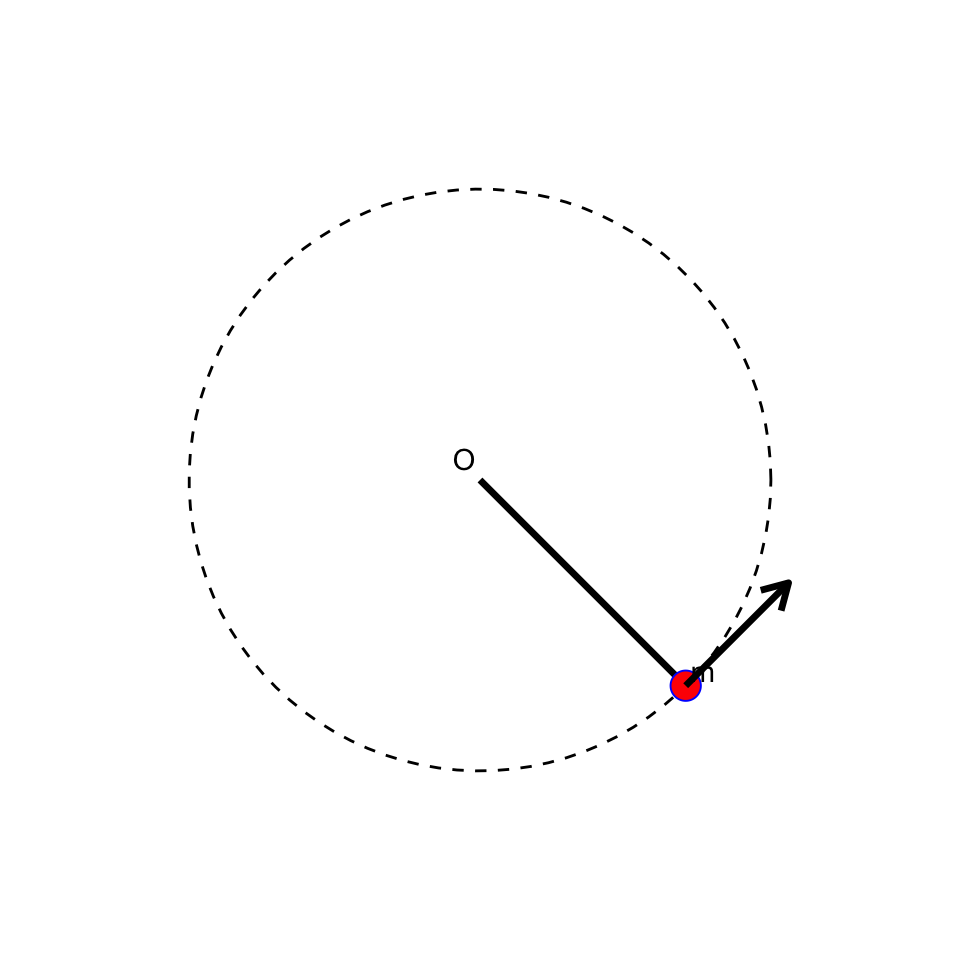
The pendulum consists of a mass m attached to a rigid, massless rod of length 1. The system is described using Cartesian coordinates (x, y), where x and y represent the horizontal and vertical positions of the mass, respectively.
Kinetic energy: T(t) = \frac{1}{2}m \left( x'(t)^2 + y'(t)^2 \right).
Potential energy: V(t) = m g y(t), where g is the gravitational acceleration.
Constraint Equation
The pendulum is constrained to move along a circular path of radius 1. This constraint is expressed as: \Phi(x, y) = x^2 + y^2 - 1 = 0.
Equations of Motion
Using Lagrange’s equations with constraints, the equations of motion for the pendulum are:
\left\{ \begin{aligned} m x''(t) + 2x(t)\lambda(t) &= 0, \\[0.5em] m y''(t) + 2y(t)\lambda(t) &= -m g, \\[0.5em] x(t)^2 + y(t)^2 &= 1, \end{aligned} \right. \tag{18.1}
where \lambda(t) is the Lagrange multiplier enforcing the constraint.
18.4 Numerical Solution
To solve the system numerically Equation 18.1, we differentiate the constraint equation twice to incorporate the acceleration terms x''(t) and y''(t).
First Derivative of the Constraint
Differentiating \Phi(x, y) = 0 once with respect to time yields: 2x(t)x'(t) + 2y(t)y'(t) = 0.
Second Derivative of the Constraint
Differentiating again gives: 2x(t)x''(t) + 2y(t)y''(t) + 2x'(t)^2 + 2y'(t)^2 = 0.
This equation introduces the acceleration terms x''(t) and y''(t), allowing us to solve for \lambda(t).
The system of equations can be written in matrix form as:
\begin{pmatrix} m & 0 & 2x(t) \\ 0 & m & 2y(t) \\ 2x(t) & 2y(t) & 0 \end{pmatrix} \begin{pmatrix} x''(t) \\ y''(t) \\ \lambda(t) \end{pmatrix} = \begin{pmatrix} 0 \\ -mg \\ -2x'(t)^2 - 2y'(t)^2 \end{pmatrix}.
Time Discretization
Given initial conditions x_0, y_0, x'_0, and y'_0, we solve the system iteratively using the following steps:
Solve for x''_k, y''_k, and \lambda_k: \begin{pmatrix} m & 0 & 2x_k \\ 0 & m & 2y_k \\ 2x_k & 2y_k & 0 \end{pmatrix} \begin{pmatrix} \color{red} x''_k \\ \color{red} y''_k \\ \color{red} \lambda_k \end{pmatrix} = \begin{pmatrix} 0 \\ -mg \\ -2(x'_k)^2 - 2(y'_k)^2 \end{pmatrix}.
Update position and velocity: \begin{aligned} x_{k+1} &= x_k + \Delta t \, x'_k + \frac{\Delta t^2}{2} \color{red} x''_k, \\ y_{k+1} &= y_k + \Delta t \, y'_k + \frac{\Delta t^2}{2} \color{red} y''_k, \\ x'_{k+1} &= x'_k + \Delta t \, \color{red} x''_k, \\ y'_{k+1} &= y'_k + \Delta t \, \color{red} y''_k. \end{aligned}
Numerical solution shows that the numerical method do not work well
19 Baumgarte’s stabilization
A very popular way to stabilize the constraint \bm{\phi}(\bm{p},t)=0 and thus avoid the drift effect is using Baumgarte’s stabilization, see [2]. This idea is well presented with other techniques in the survey paper [1]. The key idea is to substitute the constraint with a differential equation that asymptotically satisfies \bm{\phi}(\bm{p},t)=0. Obviously this technique is effective only if you are interested in the long term behaviour, since during transients the constraint may be violated. Since constrained mechanical systems require to differentiations to eliminate the Lagrange multipliers, we consider a linear second order stable differential equation of the form,
\frac{\mathrm{d}^2 z(t)}{\mathrm{d} t^2} + 2\xi\omega_{\textnormal{n}}\frac{\mathrm{d} z(t)}{\mathrm{d} t} + \omega_{\textnormal{n}}^2z(t) = 0, \tag{19.1}
where z(t)\in\Bbb{R}. In this form we recognize the well known equation for second order linear mechanical or electrical systems, such as the RLC circuit or the mass spring damper. In these framework \xi\in\Bbb{R}_{>0} is the damping ratio and \omega_{\textnormal{n}}\in\Bbb{R}_{>0} is the natural frequency. Depending on the value of \xi different cases can arise:
- 0<\xi<1: solution z is underdamped,
- \xi=1: solution z is critically damped,
- \xi>1: solution z is overdamped.
The general form for the solution is the following
z(t) = k_{1}e^{\left(-\xi+\sqrt{\xi^2-1}\right)\omega_{\text{n}}t} + k_{2}e^{\left(-\xi-\sqrt{\xi^2-1}\right)\omega_{\text{n}}t},
where k_{1},k_{2}\in\Bbb{R} are constants determined by the initial conditions z_{0} = z(t=0) and \dot{z}_{0} = \dot{z}(t=0). Solutions for the different cases can be arranged in different ways, here we show some of them. For a deeper treatment see for example [3]. Let us start from the underdamped case; solution takes the form
z(t) = c_ {1}e^{-\xi\omega_{\textnormal{n}}t} \cos\left({\sqrt{1-\xi^2}\omega_{\textnormal{n}}t-c_{2}}\right), \tag{19.2}
where constants c_{1},c_{2}\in\Bbb{R} are given by,
\begin{aligned} c_{1} &= \frac{\sqrt{z_{0}^2 \omega_{\textnormal{n}}^2+\dot{z}_{0}^2+2z_{0}\dot{z}_{0}\xi \omega_{\textnormal{n}}}}{\sqrt{1-\xi^2}\omega_{\textnormal{n}}} \\ c_{2} &= \mathrm{arctan}\left(\frac{\dot{z}_{0}+\xi\omega_{\textnormal{n}}z_{0}} { x_ {0}\omega_{\textnormal{n}}\sqrt{1-\xi^2}}\right). \end{aligned}
As we can observe in Equation 19.2 solution is a cosine function modulated by a decreasing exponential function. For the critically damped case a linear term appears and the solution takes the form,
z(t) = (c_{1}+c_{2}t)e^{-\omega_{\textnormal{n}}t}, \tag{19.3}
where c_{1},c_{2}\in\Bbb{R} are given by c_{1} = z_{0} and c_{2} = \dot{z}_{0}+\omega_{\textnormal{n}}z_{0}. Finally for the overdamped case the solution takes the form
z(t) = c_{1}e^{\left(-\xi+\sqrt{\xi^2-1}\right)\omega_{\textnormal{n}}t} + c_{2}e^{\left(-\xi-\sqrt{\xi^2-1}\right)\omega_{\textnormal{n}}t}, \tag{19.4}
with constants,
\begin{aligned} c_{1} &= \frac{x_{0}\omega_{\textnormal{n}} \left(\xi+\sqrt{\xi^2-1}\right)+\dot{x}_{0}}{2\omega_{\textnormal{n}}\sqrt{\xi^2-1}}, \\ c_{2} &= \frac{-x_{0}\omega_{\textnormal{n}} \left(\xi-\sqrt{\xi^2-1}\right)-\dot{x}_{0}}{2\omega_{\textnormal{n}}\sqrt{\xi^2-1}}. \end{aligned}
However, regardless of the specific form of the solution, all the three cases satisfy a global exponential stability property, i.e., \forall(z_{0},\dot{z}_{0})\in\Bbb{R}\times\Bbb{R} the solution z(t,z_{0},\dot{z}_{0}) satisfies
\lim_{t\rightarrow\infty} z(t,z_{0},\dot{z}_{0}) = 0.
The notation z(t,z_{0},\dot{z}_{0}) is just to stress that the solution depends on time but also from initial conditions (z_{0},\dot{z}_{0}). This consideration suggests to substitute the constraint \bm{\phi}(\bm{p},t) with an ODE of the form Equation 19.1. In this way, despite the initial conditions, the solution will asymptotically satisfies \bm{\phi}(\bm{p},t)=0. Thus the explicit Baumgarte’s stabilization for DAEs of index three takes the form,
\frac{\mathrm{d}^2\bm{\phi}}{\mathrm{d} t^2} + 2\xi\omega_{\textnormal{n}}\frac{\mathrm{d}\bm{\phi}}{\mathrm{d} t} + \omega_{\textnormal{n}}^2\bm{\phi} = 0.
Computing explicitly the terms for mechanical systems the stabilization results,
\frac{\mathrm{d}}{\mathrm{d} t}\frac{\partial\bm{\phi}} {\partial\bm{p}}\dot{\bm{p}}+\frac{\partial\bm{\phi}} {\partial\bm{p}}\ddot{\bm{p}}+\frac{\partial^{2}\bm{\phi}} {\partial t^2} + 2\xi\omega_{\textnormal{n}} \frac{\partial\phi}{\partial\bm{p}}\dot{\bm{p}} + 2\xi\omega_{\textnormal{n}}\frac{\partial\bm{\phi}}{\partial t}+\omega_{\textnormal{n}}^2\bm{\phi} = 0.
which can be re-arranged in the following form
\begin{aligned} -\frac{\partial\bm{\phi}}{\partial\bm{p}}\dot{\bm{v}} & = \frac{\mathrm{d}}{\mathrm{d} t}\frac{\partial\bm{\phi}}{\partial\bm{p}}\bm{v} +\frac{\partial^{2}\bm{\phi}}{\partial t^2} + 2\xi\omega_{\textnormal{n}}\frac{\partial\phi}{\partial\bm{p}}\bm{v} + 2\xi\omega_{\textnormal{n}}\frac{\partial\bm{\phi}}{\partial t} +\omega_{\textnormal{n}}^2\bm{\phi} \\ & =\bm{m}(\bm{p},\bm{v},t). \end{aligned} \tag{19.5}
Now Equation 19.5 can be easy implemented without any modification in Equation 11.3; indeed it is sufficient to redefine \bm{m}(\bm{p},\bm{v},t) as in Equation 19.5. However a question is still open, how can we tune the parameters \omega_{\textnormal{n}} and \xi?. Unfortunately there is not general rule, but it is useful to notice that the velocity of convergence to zero of the solution depends on both\xi and \omega_{\textnormal{n}}. Therefore it is a good idea to select them in order to obtain an high decay rate compatibly with the numerical stability. This means that the dynamics associated to the constraint \bm{\phi}(\bm{p},t) cannot be too fast compared to other ones, otherwise the system could be very hard (stiff) to simulate numerically. Indeed systems where two or more very different time scales are involved are usually called stiff problems or *stiff systems**. These may cause some numerical problems, since stiff equations require an integration step extremely small and are numerically unstable. In general it is hard to provide a unique definition of stiffness, but the main idea is that the differential equations includes some terms that can lead to rapid variation in the solution.
Example 19.1 Continuing Example 19.1} we want use the Baumgarte’s echnique to stabilize the pendulum. Therefore the idea is to substitute the constraint
2\bm{v}^{\intercal}\bm{v}+2\bm{p}\dot{\bm{v}} = 0
with
-2(\bm{p}\cdot\dot{\bm{v}}) = 2(\bm{v}\cdot\bm{v}) + 4\omega_{\textnormal{n}}\xi(\bm{p}\cdot\bm{v}) + \omega_{\textnormal{n}}^{2}(\bm{p}\cdot\bm{p}-\ell^{2}).
Thus final equations appears as,
\begin{bmatrix} \bm{I} & 0 & 0 \\ 0 & m\bm{I} & -2\bm{p} \\ 0 & -2\bm{p}^T & 0 \end{bmatrix} \begin{bmatrix} \dot{\bm{p}} \\ \dot{\bm{v}} \\ \lambda \end{bmatrix} = \begin{bmatrix} \bm{v} \\ -mg\bm{e}_{2}\\ 2(\bm{v}\cdot\bm{v}) + 4\omega_{\textnormal{n}}\xi(\bm{p}\cdot\bm{v}) + \omega_{\textnormal{n}}^{2}(\bm{p}\cdot\bm{p}-\ell^{2}) \end{bmatrix}. \tag{19.6}
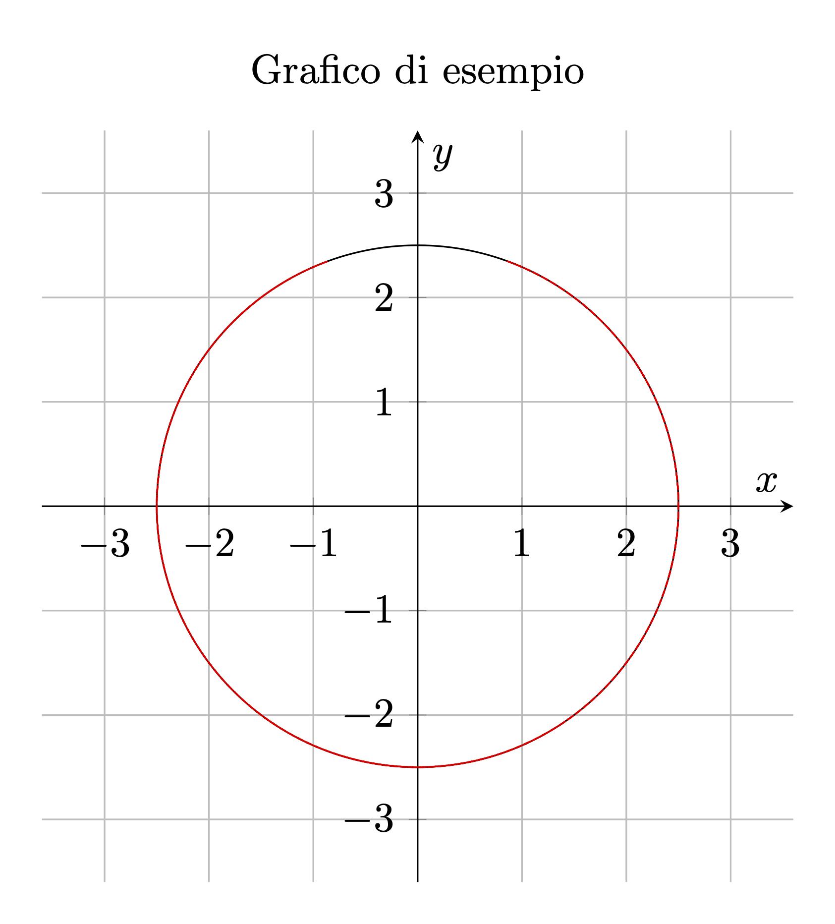
Again to appreciate the effects of Baumgarte’s stabilization we can simulate Equation 19.6 with same parameters as Example 19.1 and stabilization parameters \xi = 0.8, \omega_{\textnormal{n}} = 2. The result is showed in Figure 19.1.
Baumgarte details
The Baumgarte method stabilizes the constraints by introducing damping into the system. Consider the following ODE:
z''(t) + 2\zeta \omega z'(t) + \omega^2 z(t) = 0,
which has the solution:
z(t) = A(t) e^{-\zeta \omega t},
where A(t) depends on the initial conditions. For 0 \leq \zeta \leq 1, the solution decays exponentially without oscillation.
Over time, numerical errors can cause the system to drift away from the constraint \Phi(x, y) of Equation 18.1 where
\Phi(x, y) = x^2+y^2-1 = 0 \tag{19.7}
To mitigate this, we use the Baumgarte stabilization method, which modifies the constraint equation to include damping terms.
The stabilized constraint equation is: \frac{\mathrm{d}^2}{\mathrm{d}t^2} \Phi(x, y) + 2\zeta \omega \frac{\mathrm{d}}{\mathrm{d}t} \Phi(x, y) + \omega^2 \Phi(x, y) = 0, where \zeta and \omega are damping parameters. For Equation 19.7 this becomes: 2x x'' + 2y y'' + 2x'^2 + 2y'^2 + 4\zeta \omega (x x' + y y') + \omega^2 (x^2 + y^2 - 1) = 0.
Modified Linear System
The stabilized system is solved using the same time-stepping approach, but with the right-hand side of the linear system modified to include the stabilization terms: r_k = 2\left[(x'_k)^2 + (y'_k)^2\right] + 4\zeta \omega (x_k x'_k + y_k y'_k) + \omega^2 (x_k^2 + y_k^2 - 1).
The pendulum example illustrates the challenges of solving DAEs numerically, particularly the issue of constraint drift. The Baumgarte stabilization method effectively mitigates this drift, ensuring long-term stability of the solution. Proper choice of damping parameters \zeta and \omega is critical for achieving optimal performance.
19.1 Pendulum DAE reduced to first order
Start from the motion equations
\left\{ \begin{aligned} m x^{\prime\prime}+2x\lambda=0\\ m y^{\prime\prime}+2y\lambda+mg=0\\ x^2+y^2=1 \end{aligned} \right.
divide by m and set \mu=-2\lambda/m
\left\{ \begin{aligned} x^{\prime\prime}&=\mu x\\ y^{\prime\prime}&=\mu y-g\\ x^2+y^2&=r^2\\ \end{aligned} \right.
set u=x^{\prime} and v=y^{\prime} and transform to first order
\left\{ \begin{aligned} u^{\prime} &= \mu x\\ v^{\prime} &= \mu y-g\\ x^{\prime} &= u \\ y^{\prime} &= v \\ x^2+y^2 &= r^2 \end{aligned} \right.
Derive one time the constraint
2x x^{\prime}+2y y^{\prime}=0\quad\Longrightarrow\quad xu+yv=0
Derive another time the constraint
\begin{aligned} x\dot{u}+y\dot{v}+ \dot{x}u+\dot{y}v=0\quad&\Longrightarrow\\ \mu(x^2+y^2)-gy+(u^2+v^2)=0\quad&\Longrightarrow\quad r^2\mu-gy+(u^2+v^2)=0 \end{aligned}
Derive a third time the constraint obtaining a differential equation for \mu:
\begin{aligned} r^2\dot{\mu}-gv+2(u\dot{u}+v\dot{v})&=0\quad\Longrightarrow\\ r^2\dot{\mu}-gv+2\mu(ux+vy)-2gv&=0\quad\Longrightarrow\\ r^2\dot{\mu}-3gv&=0 \end{aligned}
The DAE has index 3
NoteSummary
Original DAE
\left\{ \begin{aligned} u^{\prime}&=\mu x\\ v^{\prime}&=\mu y-g\\ x^{\prime}&=u \\ y^{\prime}&=v \\ x^2+y^2&=1 \end{aligned} \right.
hidden constraints
\begin{aligned} xu+yv & = 0\\ \mu-gy+(u^2+v^2)&=0 \end{aligned}
constraint differential equation
\mu^{\prime}-3gv=0
19.2 Integration of the DAE without stabilization
Consider the ODE without stabilization
\left\{ \begin{aligned} u^{\prime} &= \mu x\\[0.25em] v^{\prime} &= \mu y - g\\[0.25em] x^{\prime} &= u \\[0.25em] y^{\prime} &= v \\[0.25em] \mu^{\prime}&=3gv/r^2 \end{aligned} \right.
Integration with implicit Euler:
\begin{aligned} \frac{u_{k+1}-u_{k}}{h}&=\mu_{k+1}x_{k+1}\\ \frac{v_{k+1}-v_{k}}{h}&=\mu_{k+1}y_{k+1}-g \\ \frac{x_{k+1}-x_{k}}{h}&=u_{k+1} \\ \frac{y_{k+1}-y_{k}}{h}&=v_{k+1} \\ \color{blue}\frac{\mu_{k+1}-\mu_{k}}{h}&\color{blue}=\frac{3gv_{k+1}}{r^2} \end{aligned}
Solving the first four equations for x_{k+1}, y_{k+1}, u_{k+1} and v_{k+1}
\begin{aligned} c_{k+1}&= 1-h^2\mu_{k+1} \\[0.25em] x_{k+1}&=(x_k+hu_k)/c_{k+1} \\[0.25em] y_{k+1}&=(y_k+h v_k-gh^2)/c_{k+1} \\[0.25em] u_{k+1}&=(u_k+h\mu_{k+1}x_k)/c_{k+1} \\[0.25em] v_{k+1}&=(v_k+h\mu_{k+1}y_k-gh)/c_{k+1} \end{aligned}
substituting into the multiplier equation and set \delta=\mu_{k+1}-\mu_k a quadratic in \delta is obtained:
r^2h^2\delta^2 +(3gh^2y_k+r^2(h^2\mu_k-1))\delta+3gh(v_k+y_k\mu_kh-gh)=0
Choose for the solution the \delta closer to the esplicit step, i.e. \delta\approx 3hgv_k/r^2
Implicit Eulero implicito without stabilization do not work. The constraint x^2+y^2=1 is violated in few steps:
onsider the DAE without stabilization
\left\{ \begin{aligned} u^{\prime} &= \mu x\\[0.25em] v^{\prime} &= \mu y - g\\[0.25em] x^{\prime} &= u \\[0.25em] y^{\prime} &= v \\[0.25em] \color{blue} x^2+y^2&\color{blue}=r^2 \end{aligned} \right.
Using implicit Euler:
\begin{aligned} \frac{u_{k+1}-u_{k}}{h}&=\mu_{k+1}x_{k+1}\\ \frac{v_{k+1}-v_{k}}{h}&=\mu_{k+1}y_{k+1}-g \\ \frac{x_{k+1}-x_{k}}{h}&=u_{k+1} \\ \frac{y_{k+1}-y_{k}}{h}&=v_{k+1} \\ \color{blue} x_{k+1}^2+y_{k+1}^2 & \color{blue} = 1 \end{aligned}
Solving the first four equation for x_{k+1}, y_{k+1}, u_{k+1} and v_{k+1}
\begin{aligned} c_{k+1}&= 1-h^2\mu_{k+1} \\[0.25em] x_{k+1}&=(x_k+hu_k)/c_{k+1} \\[0.25em] y_{k+1}&=(y_k+h v_k-gh^2)/c_{k+1} \\[0.25em] u_{k+1}&=(u_k+h\mu_{k+1}x_k)/c_{k+1} \\[0.25em] v_{k+1}&=(v_k+h\mu_{k+1}y_k-gh)/c_{k+1} \end{aligned}
substituting into constraint a quadratic equation in \mu_{k+1} is obtained:
x_k^{2}+y_k^2-r^2 +2 h (x_k u_k+y_0 v_k) +h^2 (u_k^2+v_k^2) \\[1em] +g^2 h^4 -2 g h^2 (y_k+h v_k)+2h^2\mu_{k+1}-h^4\mu_{k+1}^2=0
\begin{aligned} \underbrace{[x_k^{2}+y_k^2-r^2]}_{A} +2 h \underbrace{(x_k u_k+y_0 v_k)}_{B} +h^2 (u_k^2+v_k^2) \\ +g^2 h^4 -2 g h^2 (y_k+h v_k)+2h^2\mu_{k+1}-h^4\mu_{k+1}^2=0 \end{aligned}
On the solution block (A) is zero so it is removed. Block (B) is the constraint derivative not 0 in the discretization. Thus,
2 (x_k u_k+y_0 v_k) +h (u_k^2+v_k^2) +g^2 h^3 -2 g h (y_k+h v_k)+2h\mu_{k+1}-h^3\mu_{k+1}^2=0
Solving the quadratic
\begin{aligned} \mu_{k+1}&=\frac{r\pm\sqrt{r^2+A}}{h^2r}\\[1em] A &= g^2h^4+2h(x_ku_k+y_kv_k)-2gh^2(y_k-hv_k)+h^2(u_k^2+v_k^2) \end{aligned}
\mu represent centripetal force maintaining mass on the constraint. Thus \mu must be negative and solving trying to avoid cancellation error:
\begin{aligned} A &= g^2h^4+2h(x_ku_k+y_kv_k)-2gh^2(y_k-hv_k)+h^2(u_k^2+v_k^2)\\[1em] \mu_{k+1}&=\frac{-A}{h^2(r^2+r\sqrt{r^2+A})} %%=\frac{-A}{h^2(r^2+r^2\sqrt{1+A/r^2})} =\frac{-A/r^2}{h^2(1+\sqrt{1+A/r^2})} \end{aligned}
Numerical Results
19.3 Baumgarte stabilization
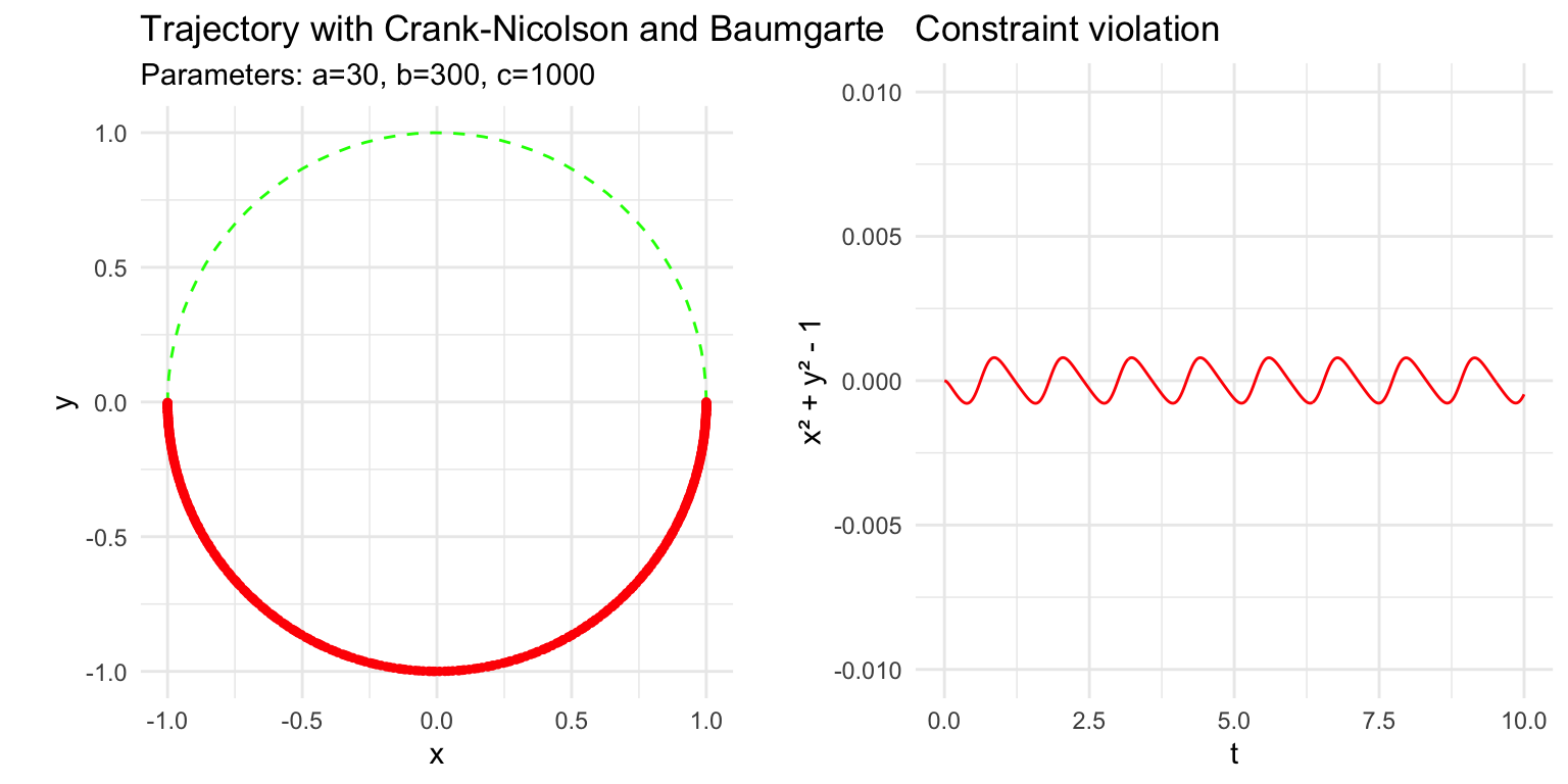
Inplicit Euler work but it is too dissipative. Cranck-Nicolson needs stabilization. DAE transformed to ODE need a third order ODE to stabilize as follows:
\dfrac{\mathrm{d}^3 V(x,y)}{\mathrm{d}t^3} +a\dfrac{\mathrm{d}^2 V(x,y)}{\mathrm{d}t^2} +b\dfrac{\mathrm{d} V(x,y)}{\mathrm{d}t} +cV(x,y)=0
where V(x,y)=x^2+y^2-1. And a, b, c are chosen in such a way
z'''(t)+az''(t)+bz'(t)+cz(t)=0
satisfy \lim_{t\to\infty}z(t)=0.
Results with Crank-Nicolson