13 Index reduction of a NonLinear DAE

This tutorial explains how to compute the index of a non-linear DAE systematically.
13.1 General DAE
A general Differential-Algebraic equation (DAE) takes the form:
\bm{f}(\bm{x},\bm{x}^\prime,t) = \bm{0},
where
- \bm{x} represents the state variables
- \bm{x}^\prime denotes their derivatives with respect to time t
- \bm{f} is a system of equations involving both algebraic and differential components.
The defining characteristic of a DAE is that the Jacobian matrix
\dfrac{\partial \bm{f}(\bm{x},\bm{x}^\prime,t)}{\partial \bm{x}^\prime}
is singular, meaning that the system does not explicitly define all derivatives in terms of the state variables. This is in contrast to ordinary differential equations (ODEs), where the system can be solved explicitly for \bm{x}^\prime.
13.2 Semi-Explicit Form of DAEs
Introducing the auxiliary variable \bm{y} = \bm{x}^\prime, the DAE can be rewritten as the system:
\left\{ \begin{aligned} \bm{x}^\prime &= \bm{y}, \\ \bm{0} &= \bm{f}(\bm{x},\bm{y},t). \end{aligned} \right.
This is a special case of the semi-explicit DAE of the form:
\left\{ \begin{aligned} \bm{x}^\prime &= \bm{g}(\bm{x},\bm{y},t), \\ \bm{0} &= \bm{f}(\bm{x},\bm{y},t), \end{aligned} \right.
where \bm{g} defines an explicit relationship for the differential variables.
13.3 Matrix Representation
The semi-explicit DAE system can be expressed in a compact matrix form:
\underbrace{ \begin{pmatrix} \bm{I} & \bm{0} \\ \bm{0} & \bm{0} \end{pmatrix} }_{\bm{\mathcal{E}}(\bm{z},t)} \, \underbrace{ \begin{pmatrix} \bm{x}^\prime \\ \bm{y}^\prime \end{pmatrix} }_{\bm{\mathcal{z}}(t)} = \underbrace{ \begin{pmatrix} \bm{g}(\bm{x},\bm{y},t) \\ \bm{f}(\bm{x},\bm{y},t) \end{pmatrix} }_{\bm{\mathcal{G}}(\bm{z},t)}.
This formulation aligns with the general form of a DAE system:
\bm{\mathcal{E}}(\bm{z},t)\,\bm{z}(t) = \bm{\mathcal{G}}(\bm{z},t),
where \bm{\mathcal{E}}(\bm{z},t) is a singular matrix, reinforcing the differential-algebraic nature of the system.
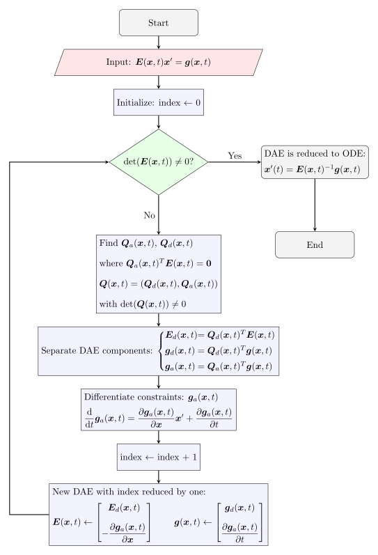
13.4 Steps to Compute the Index of a nonlinear DAE
The differential index of a differential-algebraic equation (DAE) provides insight into the complexity of solving the system. The following steps outline an approach to determine the index and perform index reduction when necessary.
Step 1: Express the DAE in Matrix Form
A nonlinear DAE can be written as:
\bm{E}(\bm{x},t) \bm{x}^\prime = \bm{g}(\bm{x},t),
where:
- \bm{E}(\bm{x},t) is an n \times n matrix,
- \bm{x}(t) represents the state variables,
- \bm{x}^\prime is the time derivative of \bm{x},
- \bm{g}(\bm{x},t) is a given function.
This formulation allows us to analyze the structure of the system and determine if it contains purely algebraic constraints.
Step 2: Check if \bm{E}(\bm{x},t) is Singular
Compute the determinant:
- If \det(\bm{E}(\bm{x},t)) \neq 0, then \bm{E}(\bm{x},t) is invertible, and the system reduces to an ODE (index 0). Terminate the procedure.
- If \det(\bm{E}(\bm{x},t)) = 0, then \bm{E}(\bm{x},t) is singular, indicating that algebraic constraints are present. Proceed to the next step.
Remark 13.1 (Constant Rank Assumption). We assume that \bm{E}(\bm{x},t) has constant rank in the domain of interest (\bm{x},t). If the rank varies, numerical methods must adapt accordingly, and the system’s index may change dynamically.
Step 3: Decompose the System into Differential and Algebraic Parts
Determine the rank of \bm{E}(\bm{x},t), denoted as r = \operatorname{rank}(\bm{E}). Define:
A basis \bm{Q}_a(\bm{x},t) \in \Bbb{R}^{n \times (n-k)} for the null space \mathcal{N}(\bm{E}(\bm{x},t)^T), which identifies the algebraic constraints. This basis satisfies: \bm{E}(\bm{x},t)^T\bm{Q}_a(\bm{x},t) = \bm{0}, \quad \text{or equivalently,} \quad \bm{Q}_a(\bm{x},t)^T\bm{E}(\bm{x},t) = \bm{0}.
A matrix \bm{Q}_d(\bm{x},t) \in \Bbb{R}^{n \times k} that completes \bm{Q}_a(\bm{x},t) to a full basis, ensuring that: \bm{Q}(\bm{x},t) = \begin{pmatrix} \bm{Q}_d(\bm{x},t), \bm{Q}_a(\bm{x},t) \end{pmatrix} is non-singular.
By multiplying the original system by \bm{Q}(\bm{x},t)^T, we obtain:
Differential part: \color{blue} \bm{E}_d(\bm{x},t) \bm{x}^\prime = \bm{g}_d(\bm{x},t), where: \bm{E}_d(\bm{x},t) = \bm{Q}_d(\bm{x},t)^T \bm{E}(\bm{x},t), \quad \bm{g}_d(\bm{x},t) = \bm{Q}_d^T(\bm{x},t)\bm{g}(\bm{x},t).
Algebraic part: \color{blue} \bm{g}_a(\bm{x},t) = \bm{0}, where: \bm{g}_a(\bm{x},t) = \bm{Q}_a(\bm{x},t)^T\bm{g}(\bm{x},t). Since \bm{Q}_a(\bm{x},t)^T \bm{E}(\bm{x},t) = \bm{0}, no derivatives appear in this equation.
Step 4: Differentiate the Algebraic Constraints
The algebraic constraints must be differentiated to reveal hidden differential equations:
\frac{\mathrm{d}}{\mathrm{d}t} \bm{g}_a(\bm{x},t) = \bm{g}_a^t(\bm{x},t) + \bm{g}_a^x(\bm{x},t) \bm{x}^\prime(t) = \bm{0}.
Rewriting, the system becomes:
\begin{pmatrix} \bm{E}_d(\bm{x},t) \\ -\bm{g}_a^x(\bm{x},t) \end{pmatrix} \bm{x}^\prime = \begin{pmatrix} \bm{g}_d(\bm{x},t) \\ \bm{g}_a^t(\bm{x},t) \end{pmatrix}.
Defining:
\widetilde{\bm{E}}(\bm{x},t) = \begin{pmatrix} \bm{E}_d(\bm{x},t) \\ -\bm{g}_a^x(\bm{x},t) \end{pmatrix}, \quad \widetilde{\bm{g}}(\bm{x},t) = \begin{pmatrix} \bm{g}_d(\bm{x},t) \\ \bm{g}_a^t(\bm{x},t) \end{pmatrix},
we obtain a new DAE system:
\widetilde{\bm{E}}(\bm{x},t) \bm{x}^\prime = \widetilde{\bm{g}}(\bm{x},t).
Step 5: Repeat Until \widetilde{\bm{E}}(\bm{x},t) Becomes Non-Singular
Repeat Steps 2–4 until \widetilde{\bm{E}}(\bm{x},t) is invertible. The differentiation index is the number of times Step 4 is performed before reaching an ODE system.