11 Numerical Integration of DAE

As pointed out in [1], both from a theoretical and numerical point of view, DAEs are much more challenging than ordinary differential equations (ODEs). Some DAEs can be solved using numerical methods for stiff systems, but others cannot, and they are very sensitive to the step size, which may lead to large errors in the solution and numerical instability. For DAEs arising from constrained mechanical systems, a fairly general form is the following:
\left\{ \begin{aligned} \bm{M}(\bm{q},\bm{q}',t)\bm{q}'' - \frac{\partial\bm{\phi}(\bm{q}, t)}{\partial\bm{q}}^T \bm{\lambda} &= \bm{n}(\bm{q},\bm{q}', t), \\[0.5em] \bm{\phi}(\bm{q}, t) &= 0 \end{aligned} \right.
where the term
\bm{n}(\bm{q},\bm{q}', t) \in \Bbb{R}^{n}
collects all the contributions coming from Coriolis and centrifugal effects, conservative and non-conservative forces. It can be defined as follows:
\bm{n}(\bm{q},\bm{q}', t) = \bm{\tau} - \bm{C}(\bm{q},\bm{q}') \bm{q}' - \bm{g}(\bm{q}).
It is well known that the equations of motion for a mechanical system are a system of second-order (possibly non-linear) differential equations. However, for clarity and generality, it is useful to consider a first-order representation. For this purpose, let us define \bm{v} \in \Bbb{R}^{n} as generalized velocities, i.e.,
\bm{v} := \bm{q}'.
Thus, substituting the above equation into the general form of the equation of motion results in:
\left\{ \begin{aligned} \bm{q}' &= \bm{v}, \\[1em] \bm{M}(\bm{q},\bm{v},t)\bm{v}' - \frac{\partial\bm{\phi}(\bm{q}, t)}{\partial\bm{q}}^T \bm{\lambda} &= \bm{n}(\bm{q}, \bm{v}, t), \\[1em] \bm{\phi}(\bm{q}, t) &= 0. \end{aligned} \right. \tag{11.1}
Notice that the vector
\begin{pmatrix} \bm{q}\\ \bm{v} \end{pmatrix} \in \Bbb{R}^{2n}
represents the state of a mechanical system, namely the pair of generalized position and generalized velocity.
11.1 Reduction to ODE
Now, a good question is how to solve the problem in the equation above. The issue is how to determine the value for the Lagrange multiplier \bm{\lambda}. One possible approach is to transform the problem into a system of pure differential equations. In order to do so, we need to differentiate the constraint \bm{\phi}(\bm{q}, t), which yields:
\frac{\mathrm{d}\bm{\phi}}{\mathrm{d}t} = \frac{\partial\bm{\phi}}{\partial\bm{q}} \bm{v} + \frac{\partial\bm{\phi}}{\partial t} = \bm{0}.
Notice that when the constraint does not depend on time, this expression indicates that the generalized velocity \bm{v} must be orthogonal to the gradient of the constraint. This also provides the opportunity to note that the constraint \bm{\phi}(\bm{q}, t) imposes relationships at the velocity and acceleration levels, restricting the set of feasible velocities. The constraints that we can obtain by differentiating the constraint are sometimes called hidden constraints.
Finally, notice that the equation above is still algebraic in the \bm{v} coordinate. Thus, in order to obtain a differential relationship, let us differentiate again:
\frac{\mathrm{d}^2\bm{\phi}(\bm{q}, t)}{\mathrm{d}t^2} = \frac{\mathrm{d}}{\mathrm{d}t} \left( \frac{\partial\bm{\phi}}{\partial\bm{q}} \bm{v} \right) + \frac{\partial\bm{\phi}}{\partial\bm{q}} \bm{v}' + \frac{\partial^2\bm{\phi}}{\partial t^2} = \bm{0}.
Notice that now this expression does not impose any algebraic constraint on the state of the mechanical system (\bm{q}; \bm{v}). Substituting the constraint \bm{\phi}(\bm{q}, t) = \bm{0} with the one derived above results in the following modified problem:
\left\{ \begin{aligned} \bm{q}' &= \bm{v}, \\[1em] \bm{M}(\bm{q},\bm{v},t)\bm{v}' - \frac{\partial\bm{\phi}(\bm{v},t)}{\partial\bm{q}}^T \bm{\lambda} &= \bm{n}(\bm{q}, \bm{v}, t), \\[1em] - \frac{\partial\bm{\phi}(\bm{v},t)}{\partial\bm{q}}\bm{v}' &= \bm{m}(\bm{q}, \bm{v}, t). \end{aligned} \right. \tag{11.2}
Here, to simplify the notation, we introduce the map
\bm{m}(\bm{q}, \bm{v}, t) := \frac{\mathrm{d}}{\mathrm{d}t} \left( \frac{\partial\bm{\phi}}{\partial\bm{q}} \bm{v} \right) + \frac{\partial^2\bm{\phi}}{\partial t^2}, \quad \bm{m}(\bm{q}, \bm{v}, t) \in \Bbb{R}^m.
Even though differentiating the constraint seems promising, the problem in the above equations and the one derived earlier are not equivalent. This difference leads to the so-called drift effect, which will be discussed in the next section. For now, let’s continue along the current path. The system of equations can also be written in compact matrix notation as follows:
\begin{bmatrix} \bm{I} & \bm{0} & \bm{0} \\ \bm{0} & \bm{M}(\bm{q},\bm{v},t) & -\dfrac{\partial\bm{\phi}}{\partial\bm{q}}^T(\bm{q},t) \\ \bm{0} & -\dfrac{\partial\bm{\phi}}{\partial\bm{q}}(\bm{q},t) & \bm{0} \end{bmatrix} \begin{bmatrix} \bm{q}' \\[1em] \bm{v}' \\[1em] \bm{\lambda} \end{bmatrix} = \begin{bmatrix} \bm{v} \\[1em] \bm{n}(\bm{q}, \bm{v}, t) \\[1em] \bm{m}(\bm{q}, \bm{v}, t) \end{bmatrix}.
Now, it’s easy to see that if the matrix on the left-hand side is invertible, we can express the system in explicit form and use this representation to perform numerical simulations. The matrix is invertible if and only if the sub-block:
\begin{bmatrix} \bm{M} & -\dfrac{\partial\bm{\phi}}{\partial\bm{q}}^T \\[1em] -\dfrac{\partial\bm{\phi}}{\partial\bm{q}} & \bm{0} \end{bmatrix} \in \Bbb{R}^{(n+m)\times(n+m)},
is non-singular (i.e., full rank).
Recall that \bm{M} is positive definite (and thus non-singular), so that
\begin{bmatrix} \bm{M} & -\dfrac{\partial\bm{\phi}}{\partial\bm{q}}^T \\[1em] -\dfrac{\partial\bm{\phi}}{\partial\bm{q}} & \bm{0} \end{bmatrix} = \begin{bmatrix} \bm{I} & \bm{0} \\[1em] -\dfrac{\partial\bm{\phi}}{\partial\bm{q}}\bm{M}^{-1} & \bm{I} \end{bmatrix} \begin{bmatrix} \bm{M} & \bm{0} \\[1em] \bm{0} & \bm{D} \end{bmatrix} \begin{bmatrix} \bm{I} & -\bm{M}^{-1}\dfrac{\partial\bm{\phi}}{\partial\bm{q}}^T \\[1em] \bm{0} & \bm{I} \end{bmatrix}
where
\bm{D} = \frac{\partial\bm{\phi}}{\partial\bm{q}} \bm{M}^{-1} \frac{\partial\bm{\phi}}{\partial\bm{q}}^T
and thus the block is non-singular if \bm{D} is non-singular.
This is not generally true, but assuming that the constraints are locally linearly independent (i.e., \forall \bm{q} \in \Bbb{R}^n, \forall t):
\text{rank}\left( \frac{\partial\bm{\phi}}{\partial\bm{q}} \right) = m,
then \bm{D} is non-singular. Thus, the system can be expressed in explicit first-order form as follows:
\begin{bmatrix} \bm{q}' \\[1em] \bm{v}' \\[1em] \bm{\lambda} \end{bmatrix} = \begin{bmatrix} \bm{I} & 0 & 0 \\ 0 & \bm{M}(\bm{q},\bm{v},t) & -\dfrac{\partial\bm{\phi}}{\partial\bm{q}}^T(\bm{q},t) \\ 0 & -\dfrac{\partial\bm{\phi}}{\partial\bm{q}}(\bm{q},t) & 0 \\ \end{bmatrix}^{-1} \begin{bmatrix} \bm{v} \\[1em] \bm{n}(\bm{q}, \bm{v}, t) \\[1em] \bm{m}(\bm{q}, \bm{v}, t) \end{bmatrix}.
An explicit expression for the inverse matrix can be obtained through tedious calculations (a calculation is done when numerical simulation are done). Regardless of the specific expression for the solution, the important point to emphasize is that by differentiating the constraint, we were able to find an explicit expression for the Lagrange multipliers. For this purpose, we differentiated twice and obtained the equation:
\bm{\lambda} = -\left( \frac{\partial\bm{\phi}}{\partial\bm{q}} \bm{M}^{-1} \frac{\partial\bm{\phi}}{\partial\bm{q}}^T \right)^{-1} \left( \frac{\mathrm{d}}{\mathrm{d}t} \frac{\partial\bm{\phi}}{\partial\bm{q}} \bm{v} + \frac{\partial\bm{\phi}}{\partial\bm{q}} \bm{M}^{-1} \bm{n}(\bm{q}, \bm{v}, t) + \frac{\partial^2\bm{\phi}}{\partial t^2} \right).
Technically, mechanical systems subject to holonomic constraints are systems of differential-algebraic equations (DAEs) of differential index 3. The differential index is one plus the number of differentiations of the constraint that are needed in order to eliminate the Lagrange multipliers. Alternatively, it is the number of times that we need to differentiate the constraint in order to obtain a differential equation for the Lagrange multiplier.
11.2 The drift effect
In this section we want investigate the effects of the differentiating process done to transform problem in Equation 11.1 into problem Equation 11.2. Unfortunately this method is not priceless, indeed formally we substitute an algebraic constraint with its second derivative w.r.t time. To better understand the consequences let us consider a fictitious constraint \widetilde{\bm{\phi}}(\bm{q},t) of the form,
\widetilde{\bm{\phi}}(\bm{q},t) := \bm{\phi}(\bm{q},t)+\bm{a}_0 + \bm{a}_{1}t.
It is easy to see that consider a mechanical system subject to constraint \phi(\bm{q},t) or \widetilde{\bm{\phi}}(\bm{q},t) differentiating twice is exactly the same, i.e.,
\frac{\mathrm{d}^2\bm{\phi}}{\mathrm{d} t^2} = \frac{\mathrm{d}^2\widetilde{\bm{\phi}}}{\mathrm{d} t^2}.
This fact produces the drift effect, i.e., the original constraint \bm{\phi}(\bm{q},t) is violated with an error growing with time. This error grows in the best case linearly, but it can be faster due to numerical errors. The reason of this behaviour is the term \bm{a}_{1}t which does not have any effect in the formulation Equation 11.2. Note also that this is not an undesired effect coming from not enough precision of the numerical scheme, but it is intrinsic effect due to substitution of the constraint \bm{\phi} with its second derivative w.r.t time. A simple solution to this undesired effect is the Baumgarte’s stabilization that we will discuss in the next section.
Example 11.1 Continuing Example 11.1 we provide a first order representation for the pendulum; setting \bm{v} = \bm{q}' results,
\begin{aligned} \bm{v} &= \bm{q}',\\ m\bm{v}' + mg\bm{e}_{2} &= 2\bm{q}\lambda,\\ \bm{q}^T\bm{q} - \ell^{2} &= 0. \end{aligned}
Then in order to eliminate the Lagrange multiplier let us differentiate the constraint,
\frac{\mathrm{d}\phi}{\mathrm{d} t} = 2 \bm{q}^T\bm{v} = 0.
Notice that as expected velocity \bm{v} and position \bm{q} are orthogonal each other. Differentiating again we obtain
\frac{\mathrm{d}^{2}\phi}{\mathrm{d} t^2} = 2(\bm{q}')^T\bm{v} + 2\bm{q}^T\bm{v}' = 2\bm{v}^T\bm{v} + 2\bm{q}^T\bm{v}' = 0.
Now we can write the problem in shape of Equation 11.3,
\begin{bmatrix} \bm{I} & 0 & 0 \\[1em] 0 & m\bm{I} & -2\bm{q} \\[1em] 0 & -2\bm{q}^T & 0 \end{bmatrix} \begin{bmatrix} \bm{q}' \\[1em] \bm{v}' \\[1em] \lambda \end{bmatrix} = \begin{bmatrix} \bm{v} \\[1em] -mg\bm{e}_{2}\\[1em] 2\bm{v}^T\bm{v} \end{bmatrix}, \tag{11.3}
where \bm{I}\in\Bbb{R}^{2\times 2} is the identity matrix of dimension 2. The explicit value for the Lagrange multipliers is the following
\lambda = -\frac{m}{2\bm{q}^T\bm{q}} \left(\bm{v}^T\bm{v}-g\bm{q}^T\bm{e}_{2}\right) = -\frac{m}{2\ell^{2}}\left(\bm{v}^T\bm{v}-gq_{2}\right). \tag{11.4}
To better appreciate the drift effect we can simulate Equation 11.3 using an ODE solver. The results are showed in Figure 11.1
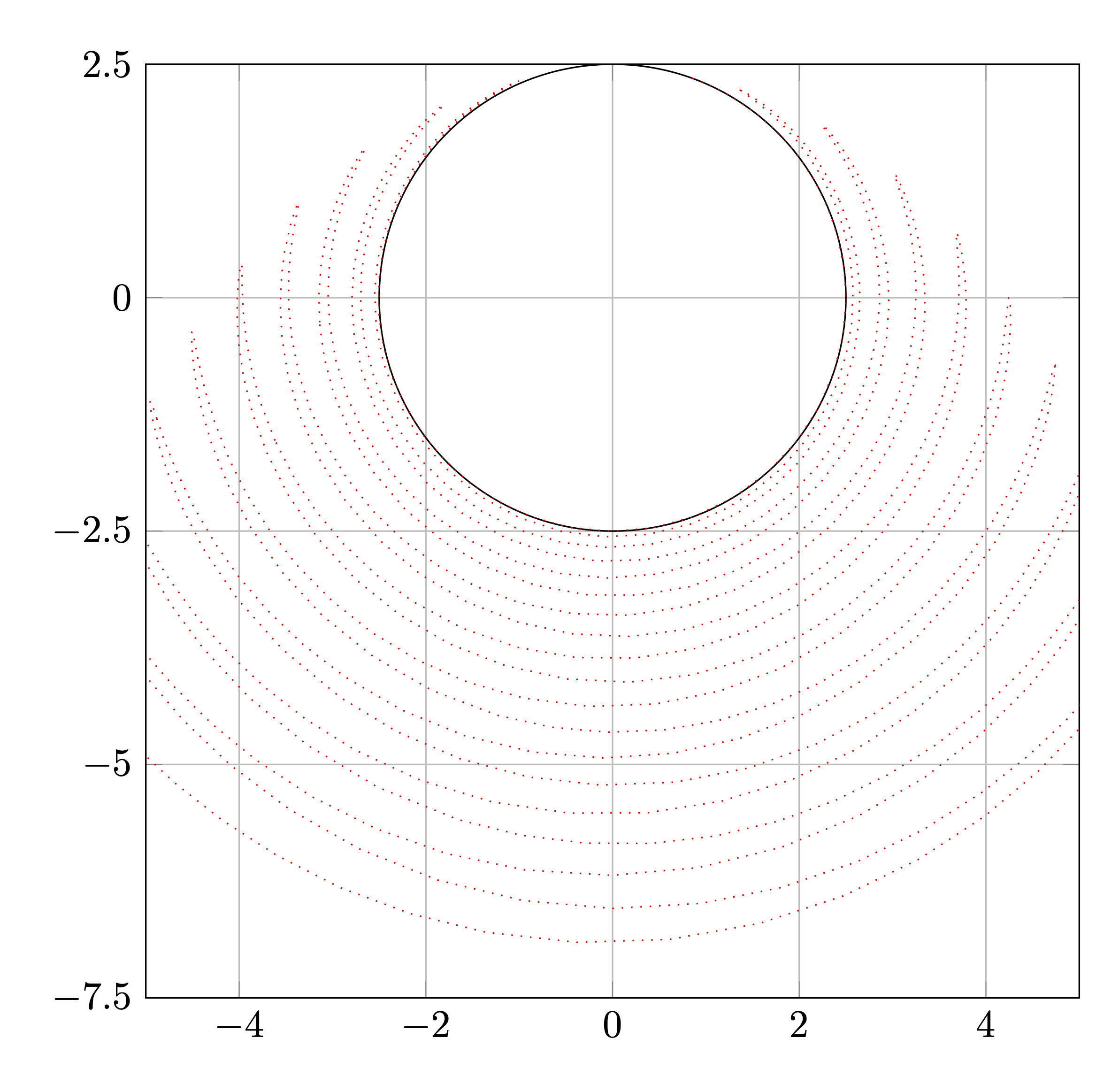
Simulation has been performed for 50 seconds with the following parameters,
- g = 9.81
- m=2
- \ell=2.5
and initial conditions
- \bm{q}_{0} = (0.86; 2.35)\in\Bbb{R}^{2},
- \bm{q}'_{0} = \bm{v}_{0} = (0,0)\in\Bbb{R}^{2}
- and \lambda_{0} = 3.69
which are all consistent with the constraint and with Equation 11.4.