
10 DAE from Lagrangian mechanics
10.1 Overview of Lagrangian Mechanics
This section primarily draws from the foundational works of [1] and [2]. Mechanics explores the behavior of systems ranging from particles and rigid bodies to continuous media and field theories, such as electromagnetism and gravitation. Since Newton’s formulation in the 17th century, mechanics has evolved into two dominant frameworks: Lagrangian mechanics and Hamiltonian mechanics. Here, we focus on the essentials of Lagrangian mechanics, with further details available in [2].
At the core of Lagrangian mechanics lies the principle of stationary action (or least action), a variational approach that generalizes Newton’s second law, \bm{F} = m \bm{a}. This principle provides a powerful method for deriving equations of motion for a wide range of physical systems. While both Lagrangian and Hamiltonian mechanics share this foundation, we will restrict our discussion to systems with a finite number of degrees of freedom.
Generalized Coordinates and Energies
For such systems, the configuration is described by a set of generalized coordinates:
\bm{q} := (q_{1}, q_{2}, \dots, q_{n}) \in \Bbb{R}^{n},
where n is the minimum number of independent variables needed to specify the system’s state. The choice of \bm{q} is not unique; different sets of generalized coordinates may describe the same system.
Given a coordinate system \bm{q}, we express
- the system’s kinetic energy T(\bm{q}, \dot{\bm{q}})
- and potential energy U(\bm{q}, t)
as functions of these variables. The kinetic energy depends on both positions \bm{q} and velocities \dot{\bm{q}}, while the potential energy generally depends on positions and may also explicitly depend on time t:
T: \Bbb{R}^{n} \times \Bbb{R}^{n} \to \Bbb{R}_{\geq 0}, \quad U: \Bbb{R}^{n} \times \Bbb{R} \to \Bbb{R}.
Though \bm{q} may parametrize more complex geometries (i.e., manifolds), in many practical cases, the configuration space can be locally approximated as Euclidean.
The Lagrangian Function
The Lagrangian function, L(\bm{q}, \dot{\bm{q}}, t), is defined as the difference between kinetic and potential energy:
L(\bm{q}, \dot{\bm{q}}, t) := T(\bm{q}, \dot{\bm{q}}) - U(\bm{q}, t). \tag{10.1}
This function encapsulates the entire dynamics of the system and serves as the foundation for the Lagrangian formulation. Its domain consists of positions, velocities, and time:
L: \Bbb{R}^{n} \times \Bbb{R}^{n} \times \Bbb{R} \to \Bbb{R}.
Euler-Lagrange Equations
The equations of motion follow from the Euler-Lagrange equations, derived by applying the principle of stationary action:
\frac{\mathrm{d}}{\mathrm{d}t} \left( \frac{\partial L}{\partial \dot{q}_{i}} \right) - \frac{\partial L}{\partial q_{i}} = 0, \quad i = 1, \dots, n.
These equations provide a systematic method for obtaining the equations of motion for mechanical systems, from simple particles to more complex rigid-body dynamics.
The Lagrangian framework offers an elegant and unified approach to modeling physical phenomena, leveraging the principle of stationary action. By encoding dynamics in a single function L(\bm{q}, \dot{\bm{q}}, t), it simplifies problem-solving and provides deep insights into the structure of classical mechanics.
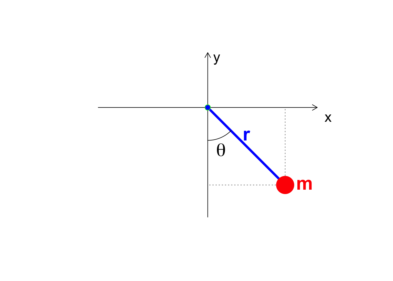
Example 10.1 (Lagrangian Mechanics in Different Coordinate Systems) Consider a free mass m moving in a plane under the influence of gravity, which acts downward along the y-axis (see Figure 10.1).
Cartesian Coordinates
In Cartesian coordinates \bm{q} = (x, y) \in \Bbb{R}^2, the kinetic and potential energies of the system are given by:
T = \frac{1}{2} m (\dot{x}^2 + \dot{y}^2), \quad U = mg y.
Thus, the Lagrangian is:
L = \frac{1}{2} m (\bm{\dot{q}} \cdot \bm{\dot{q}}) - mg (\bm{e} \cdot \bm{q}),
where \bm{e}_2 = (0, 1) is the unit vector in the y-direction.
Transformation to Polar Coordinates
Cartesian coordinates are not the only possible choice. Using polar coordinates (r, \theta) [rotated by 90 degree], we have the transformations:
x = r \sin\theta, \quad y = -r \cos\theta.
Differentiating with respect to time:
\dot{x} = \dot{r} \sin\theta + r (\cos\theta) \dot{\theta}, \quad \dot{y} = -\dot{r} \cos\theta + r (\sin\theta) \dot{\theta}.
Substituting these into the expressions for kinetic and potential energy:
T = \frac{1}{2} m (\dot{r}^2 + r^2 \dot{\theta}^2), \quad U = -mg r \cos\theta.
Thus, in the generalized coordinates \widetilde{\bm{q}} = (r, \theta), the Lagrangian takes the form:
L = \frac{1}{2} m (\dot{r}^2 + r^2 \dot{\theta}^2) + mg r \sin\theta.
This example demonstrates that the choice of generalized coordinates is not unique. Depending on the problem, selecting an appropriate coordinate system can simplify calculations. However, regardless of the chosen coordinates, the Lagrangian formulation remains consistent and yields the correct equations of motion.
10.2 The Minimal Action Principle in Classical Mechanics
A fundamental concept in classical mechanics is the action S \in \Bbb{R}. The action is defined as the integral of the Lagrangian function over time, evaluated between two instants t_1 and t_2 \in \Bbb{R}:
S := \int_{t_{1}}^{t_{2}} L(\bm{q}, \dot{\bm{q}}, t)\, \mathrm{d}t. \tag{10.2}
The action is a functional, meaning it assigns a scalar value to an entire trajectory rather than a single point. Specifically, it maps a curve \bm{q}(\cdot) in the space of possible trajectories to a real number representing the system’s total action over the time interval [t_1, t_2].
Principle of Stationary Action
The principle of stationary action (or least action principle) states that the actual path taken by a system between two points in time is the one that makes the action stationary. This means that the physical trajectory \bm{q}(t) satisfies:
\delta S = 0,
where \delta S represents the first-order variation of S due to small perturbations in the path. In most cases, this condition leads to minimizing the action, but there exist scenarios where the action is stationary but not a minimum.
This principle serves as the foundation for deriving the Euler-Lagrange equations, which govern the system’s motion:
\frac{\mathrm{d}}{\mathrm{d}t} \left( \frac{\partial L}{\partial \dot{q}_{i}} \right) - \frac{\partial L}{\partial q_{i}} = 0, \quad i = 1, \dots, n.
Thus, rather than directly applying Newton’s second law, one can obtain the equations of motion by ensuring that small variations in the trajectory do not significantly change the action.
Interpretation of the Action Functional
Remark 10.1 (Action dependence). It’s important to recognize that the action S = S(\bm{q}) depends on the entire trajectory \bm{q}(t) over the time interval [t_1, t_2], not just on individual points along the path.
To clarify notation:
- We use \bm{q}(\cdot) to represent the function describing the full trajectory.
- \bm{q}(t) refers to the specific position at a given time t.
Since S is a functional, different curves \bm{q}(\cdot) generally yield different values of S. The principle of stationary action asserts that among all possible paths connecting the given endpoints, nature selects the one that makes S stationary.
Physical Implications and Broader Context
The action principle provides a unifying framework for classical mechanics and extends naturally into other areas of physics:
- In quantum mechanics, Feynman’s path integral formulation interprets the action as a phase factor in a sum over all possible trajectories.
- In general relativity, Einstein’s field equations emerge from an action principle applied to the curvature of spacetime.
- In field theory, the action integral is extended to functional over spacetime, leading to fundamental equations such as Maxwell’s equations for electromagnetism.
By shifting the focus from forces to variational principles, the action principle offers a powerful and elegant approach to understanding physical laws.
Example 10.2 (Computing the Action for a Given Trajectory) Consider a system with generalized coordinates
\bm{q} = (q_{1}, q_{2}) \in \Bbb{R}^{2}
evolving over the time interval t \in [0,1]. Suppose the Lagrangian is given by:
L = q_{1}^{2} + q_{2}^{2}.
The action functional, defined as the integral of the Lagrangian over time, takes the form:
S = \int_{0}^{1} (q_{1}^2 + q_{2}^2) \, \mathrm{d}t.
To illustrate how the choice of trajectory affects the computed action, consider the specific path:
\bm{q}(t) = (2, t).
Substituting this trajectory into the action integral:
S = \int_{0}^{1} (2^{2} + t^{2}) \, \mathrm{d}t = \int_{0}^{1} (4 + t^{2}) \, \mathrm{d}t.
Evaluating the integral:
S = \left[ 4t + \frac{t^{3}}{3} \right]_{0}^{1} = 4(1) + \frac{1^{3}}{3} - \left( 4(0) + \frac{0^{3}}{3} \right) = 4 + \frac{1}{3} = \frac{13}{3}.
This example demonstrates how different trajectories yield different action values, emphasizing the role of path selection in variational principles.
10.3 The Calculus of Variations and the Stationary Action Principle
In classical analysis, we often look for extrema—points where a function reaches a minimum or maximum. A similar idea appears in mechanics: we may ask whether a particular trajectory of a system is, in some sense, optimal. The quantity to be optimized in this context is called the action functional.
This question leads to a fundamental area of mathematics known as the calculus of variations. Unlike traditional analysis, which focuses on functions of a few variables, the calculus of variations deals with functionals—that is, functions whose inputs are other functions, such as curves or trajectories.
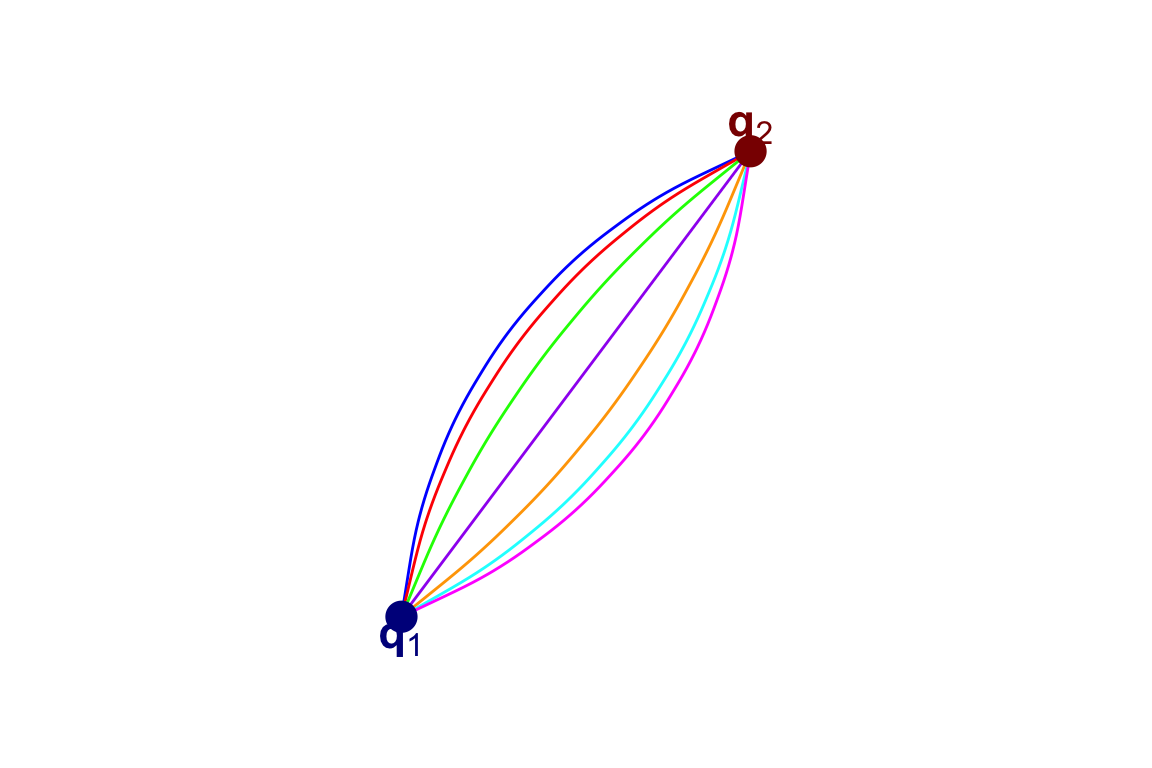
A central concept is the principle of stationary action. It states that the actual path \bm{q}(\cdot) followed by a mechanical system is one that makes the action functional stationary. This means that small variations in the path do not change the value of the action, at least to first order.
A useful analogy is that of light traveling through different media: according to Fermat’s principle, light follows the path that makes the travel time minimal. Similarly, physical systems evolve along paths that extremize (not necessarily minimize) the action.
To formalize this principle, consider a system evolving between:
- An initial time t_1, where the system is at configuration \bm{q}_1 = \bm{q}(t_1).
- A final time t_2, where the system reaches configuration \bm{q}_2 = \bm{q}(t_2).
Among all possible paths connecting \bm{q}_1 to \bm{q}_2 within the time interval [t_1, t_2], the physical trajectory satisfies:
\delta S = 0.
This variational condition (that will be discussed later in Section 10.4.2) leads directly to the Euler-Lagrange equations, which govern the motion of the system:
\frac{\mathrm{d}}{\mathrm{d}t} \left( \frac{\partial L}{\partial \dot{q}_{i}} \right) - \frac{\partial L}{\partial q_{i}} = 0, \quad i = 1, \dots, n.
Thus, the principle of stationary action provides a deep and elegant framework for deriving equations of motion across diverse physical systems, from simple particles to complex field theories.
Theorem 10.1 (Stationary Action Principle) The motion of a mechanical system evolving from configuration \bm{q}_{1} to configuration \bm{q}_{2} over a time interval t \in [t_{1}, t_{2}] follows extremal curves of the action functional, as defined in Equation 10.2. Mathematically, this means:
\delta S = 0.
where \delta S represents an infinitesimal variation in the action due to a small perturbation in the trajectory \bm{q}(\cdot). This condition implies that the physical path either minimizes, maximizes, or otherwise renders the action stationary.
A central idea in the calculus of variations is the variational operator \delta, which quantifies how a functional—such as the action—responds to small perturbations in its input. In essence, \delta serves a role analogous to that of the differential operator in classical calculus, but it acts on functionals rather than functions.
By systematically analyzing how the action varies under infinitesimal changes in the path, one obtains necessary conditions for a trajectory to make the action stationary. These conditions are precisely the Euler–Lagrange equations, which govern the motion of systems in this variational framework.
The Variational Operator: A Simple Example
Example 10.3 The concept of variation \delta is closely related to differentiation in standard calculus. To illustrate this, consider a function of two variables:
f(x, y) = \cos{x} + y^2.
A small perturbation (\delta x, \delta y) in (x, y) induces a change in f, given by:
\delta f = \frac{\partial f}{\partial x} \delta x + \frac{\partial f}{\partial y} \delta y.
Explicitly computing the partial derivatives:
\delta f = (-\sin{x}) \delta x + (2y) \delta y.
In matrix form, this can be expressed as:
\delta f = \begin{pmatrix} -\sin{x} & 2y \end{pmatrix} \begin{pmatrix} \delta x \\ \delta y \end{pmatrix}.
A stationary point of f is characterized by \delta f = 0 for all small variations. Setting the partial derivatives to zero:
\sin{x} = 0, \quad 2y = 0.
Solving for x and y gives the stationary points:
x = k\pi, \quad y = 0, \quad k \in \Bbb{Z}.
This example mirrors the variational principle in mechanics: just as stationary points of a function correspond to extrema in calculus, stationary trajectories of the action functional correspond to the actual motion of a mechanical system.
Notice that
- The calculus of variations extends classical optimization to functionals over infinite-dimensional spaces.
- The stationary action principle states that physical trajectories extremize the action functional, leading to the Euler-Lagrange equations.
- The variational operator \delta is a fundamental tool in analyzing changes in functionals, playing a role similar to differentiation in standard calculus.
By applying these principles, one can derive the laws of motion in a wide range of mechanical and physical systems, demonstrating the power and generality of Lagrangian mechanics.
10.4 Consequences of the Stationary Action Principle
The stationary action principle provides a powerful method for deriving the equations of motion of a system. If we assume that the Lagrangian L is sufficiently regular, we can exchange the order of variation and integration, allowing us to move the \delta operator under the integral sign:
\delta S = \int_{t_{1}}^{t_{2}} \delta L(\bm{q},\dot{\bm{q}},t) \, \mathrm{d}t.
Expanding the variation of L in terms of \bm{q} and \dot{\bm{q}}:
\delta S = \int_{t_{1}}^{t_{2}} \left( \frac{\partial L}{\partial \bm{q}} \delta \bm{q} + \frac{\partial L}{\partial \dot{\bm{q}}} \delta \dot{\bm{q}} \right) \mathrm{d}t. \tag{10.3}
This equation expresses the change in action due to small variations \delta \bm{q}(t) and their time derivatives \delta \dot{\bm{q}}(t).
Remark 10.2 (Fixed-Time Variations). It is important to emphasize that variations are evaluated at fixed times t_{1} and t_{2}. Consequently, the variation of L is given by:
\delta L(\bm{q}(t), \dot{\bm{q}}(t), t) = \frac{\partial L}{\partial \bm{q}} \delta \bm{q} + \frac{\partial L}{\partial \dot{\bm{q}}} \delta \dot{\bm{q}},
and does not include a term involving \delta t:
\delta L(\bm{q}(t), \dot{\bm{q}}(t), t) \neq \frac{\partial L}{\partial \bm{q}} \delta \bm{q} + \frac{\partial L}{\partial \dot{\bm{q}}} \delta \dot{\bm{q}} + \frac{\partial L}{\partial t} \delta t.
This distinction arises because time itself is not varied—only the trajectory \bm{q}(\cdot) is perturbed. Additionally, we treat \dot{\bm{q}} as an independent variable with respect to \bm{q} during the variation process.
Integration by Parts and the Euler-Lagrange Equations
A crucial step in deriving the equations of motion from the action principle involves an integration by parts. Using the identity:
\frac{\partial L}{\partial\dot{\bm{q}}} \delta\dot{\bm{q}} = \frac{\mathrm{d}}{\mathrm{d} t} \left(\frac{\partial L}{\partial\dot{\bm{q}}} \delta \bm{q} \right) - \frac{\mathrm{d}}{\mathrm{d} t} \frac{\partial L}{\partial\dot{\bm{q}}} \delta \bm{q}, \tag{10.4}
we substitute this result into equation Equation 10.3:
\begin{aligned} \delta S &= \int_{t_{1}}^{t_{2}} \left( \frac{\mathrm{d}}{\mathrm{d} t} \left(\frac{\partial L}{\partial\dot{\bm{q}}} \delta \bm{q} \right) - \frac{\mathrm{d}}{\mathrm{d} t} \frac{\partial L}{\partial \dot{\bm{q}}} \delta \bm{q} + \frac{\partial L}{\partial \bm{q}} \delta \bm{q} \right) \mathrm{d} t \\ &= \left[\frac{\partial L}{\partial\dot{\bm{q}}} \delta \bm{q}\right]_{t_{1}}^{t_{2}} + \int_{t_{1}}^{t_{2}} \left( \frac{\partial L}{\partial \bm{q}} - \frac{\mathrm{d}}{\mathrm{d} t} \frac{\partial L}{\partial\dot{\bm{q}}} \right) \delta \bm{q} \, \mathrm{d}t. \end{aligned} \tag{10.5}
The first term represents a boundary contribution that depends on the variations at the endpoints t_1 and t_2. The second integral must vanish for the action to be stationary.
Remark 10.3 (Vanishing of Boundary Terms). To ensure the physical trajectory \bm{q}(t) is uniquely determined, we impose the boundary conditions:
\delta \bm{q}(t_{1}) = \delta \bm{q}(t_{2}) = 0.
This assumption reflects the fact that the initial and final positions \bm{q}_1 and \bm{q}_2 are fixed a priori. Under this condition, the boundary term:
\left[\frac{\partial L}{\partial \dot{\bm{q}}} \delta \bm{q}\right]_{t_{1}}^{t_{2}}
vanishes, leaving us with:
\int_{t_{1}}^{t_{2}} \left( \frac{\partial L}{\partial \bm{q}} - \frac{\mathrm{d}}{\mathrm{d} t} \frac{\partial L}{\partial\dot{\bm{q}}} \right) \delta \bm{q} \, \mathrm{d}t = 0.
Since this must hold for any infinitesimal variation \delta \bm{q}, the fundamental theorem of calculus of variations implies:
\frac{\mathrm{d}}{\mathrm{d} t} \frac{\partial L}{\partial\dot{\bm{q}}} - \frac{\partial L}{\partial \bm{q}} = 0.
These are the Euler-Lagrange equations, which describe the equations of motion of the system.
Notice that
- By moving the variational operator inside the integral, we obtain an expression involving \delta \bm{q} and \delta \dot{\bm{q}}.
- Applying integration by parts, we separate boundary terms from terms inside the integral.
- The assumption \delta \bm{q}(t_1) = \delta \bm{q}(t_2) = 0 removes the boundary term, leading directly to the Euler-Lagrange equations.
These equations form the cornerstone of Lagrangian mechanics, providing a general and elegant formulation of classical mechanics.
Derivation of the Euler-Lagrange Equations
Having established the variation of the action in equation Equation 10.5, we are now in a position to simplify it further using a fundamental result from the calculus of variations.
The Fundamental Lemma of the Calculus of Variations
A crucial step in our derivation is the Fundamental Lemma of the Calculus of Variations, which allows us to extract the equations of motion from the stationary condition of the action.
Lemma 10.1 (Fundamental Lemma of Calculus of Variations) Let S be a functional in the variational sense. Suppose that for every smooth variation \delta \bm{q}(t) satisfying the boundary conditions
\delta \bm{q}(t_1) = \delta \bm{q}(t_2) = 0
we have:
\int_{t_{1}}^{t_{2}} \left( \frac{\partial L}{\partial \bm{q}} - \frac{\mathrm{d}}{\mathrm{d} t} \frac{\partial L}{\partial \dot{\bm{q}}} \right) \delta \bm{q} \, \mathrm{d}t = 0.
Then, it necessarily follows that the integrand must vanish identically:
\frac{\mathrm{d}}{\mathrm{d} t} \frac{\partial L}{\partial \dot{\bm{q}}}^{\intercal} - \frac{\partial L}{\partial \bm{q}}^{\intercal} = 0. \tag{10.6}
This result is fundamental because it allows us to conclude that if an integral of a function multiplied by an arbitrary function (the variation \delta \bm{q}) is always zero, then the function itself must be identically zero. This is a direct consequence of the fact that variations \delta \bm{q} can be chosen freely within the class of smooth functions that vanish at the endpoints.
Interpretation and Physical Meaning
The system of equations in Equation 10.6 is known as the Euler-Lagrange equations. These are the fundamental equations that govern the motion of mechanical systems within the framework of Lagrangian mechanics.
Intuitively, the fundamental lemma tells us that since the variation \delta \bm{q}(t) is arbitrary (except for vanishing at the endpoints), the only way to ensure that the integral always evaluates to zero is to have the coefficient of \delta \bm{q} vanish at every instant in time. This leads directly to the equations of motion.
Thus, we can summarize our findings in the following theorem:
Theorem 10.2 (Theorem: Euler-Lagrange Equations) The physical trajectory \bm{q}(t) of a mechanical system described by a Lagrangian L(\bm{q}, \dot{\bm{q}}, t) satisfies the system of differential equations:
\frac{\mathrm{d}}{\mathrm{d} t} \frac{\partial L}{\partial \dot{\bm{q}}}^{\intercal} - \frac{\partial L}{\partial \bm{q}}^{\intercal} = 0.
These equations provide the necessary conditions for the action functional S to be stationary under small variations of the path \bm{q}(t).
Notice that
- We derived the variation of the action integral and expressed it in terms of \delta \bm{q} and \delta \dot{\bm{q}}.
- Through integration by parts, we isolated the term involving \delta \bm{q} inside the integral and discarded the boundary terms by assuming that \delta \bm{q}(t_1) = \delta \bm{q}(t_2) = 0.
- We applied the Fundamental Lemma of the Calculus of Variations to conclude that the coefficient of \delta \bm{q} must be identically zero, leading to the Euler-Lagrange equations.
This approach not only provides a rigorous derivation but also highlights the deep connection between variational principles and the fundamental laws of motion.
10.5 Principle of Minimal Action and Coordinate Independence
The following theorem expresses the fundamental idea of the principle of stationary action:
Theorem 10.3 (Minimal Action Principle) A curve
\bm{q}: t \mapsto \bm{q}(t),\quad\text{for}\quad t \in [t_{1}, t_{2}]
is an extremal of the functional S in the space of curves that pass through the points
\bm{q}(t_{1}) = \bm{q}_{1} \quad\text{and}\quad \bm{q}(t_{2}) = \bm{q}_{2}
if and only if it satisfies the Euler-Lagrange equation:
\frac{\mathrm{d}}{\mathrm{d}t} \frac{\partial L}{\partial \dot{q}} - \frac{\partial L}{\partial q} = 0.
In practice the physical trajectory of a system is one that makes the action S stationary. In other words, among all possible paths that connect two fixed endpoints, the actual path followed by the system is the one that satisfies the Euler-Lagrange equations.
Coordinate Invariance of the Equations of Motion
A crucial feature of the Euler-Lagrange equations is their coordinate-free nature. This means that the equations remain valid regardless of the specific coordinate system chosen to describe the motion. The principle of least action, and thus the resulting equations of motion, do not depend on how we label points in space but rather on the intrinsic physics of the system.
To illustrate this, consider the case of a free particle moving under gravity, analyzed in two different coordinate systems.
Example 10.4 (Motion of a Free Mass Point in Different Coordinates) We examine the equations of motion for a particle of mass m subject to gravity in both Cartesian and polar coordinates.
Cartesian Coordinates
In Cartesian coordinates, the equations of motion follow directly from the Euler-Lagrange equations:
\frac{\mathrm{d}}{\mathrm{d}t} \frac{\partial L}{\partial \dot{q}} - \frac{\partial L}{\partial q} = m\ddot{q} + mg e_{2} = 0. \tag{10.7}
Here, e_{2} is the unit vector in the vertical direction.
Polar Coordinates
In polar coordinates (\tilde{q}_{1}, \tilde{q}_{2}), where \tilde{q}_{1} represents the radial coordinate and \tilde{q}_{2} the angular coordinate, the equations take a different form:
\begin{aligned} \frac{\mathrm{d}}{\mathrm{d}t} \frac{\partial L}{\partial \dot{\tilde{q}}_{1}} - \frac{\partial L}{\partial \tilde{q}_{1}} &= m\ddot{\tilde{q}}_{1} + mg \sin(\tilde{q}_{2}), \\ \frac{\mathrm{d}}{\mathrm{d}t} \frac{\partial L}{\partial \dot{\tilde{q}}_{2}} - \frac{\partial L}{\partial \tilde{q}_{2}} &= m\tilde{q}_{1}^{2}\ddot{\tilde{q}}_{2} + 2m\tilde{q}_{1}\dot{\tilde{q}}_{1}\dot{\tilde{q}}_{2} + mg\tilde{q}_{1}\cos(\tilde{q}_{2}) = 0. \end{aligned} \tag{10.8}
Even though the equations appear different in Cartesian and polar coordinates, they describe the same physical motion. The coordinate transformation between the two representations maintains the fundamental structure of the equations, underscoring the coordinate-free nature of Lagrangian mechanics.
Beyond Conservative Systems: Generalized Forces
One limitation of the Euler-Lagrange formulation, as presented so far, is that it applies strictly to conservative systems, where the forces derive from a potential energy function. However, many physical systems include non conservative forces, such as friction or external driving forces, which do not fit within the standard Lagrangian framework.
To extend the formulation to non conservative forces, we introduce D’Alembert’s principle, which leads to a modification of the Euler-Lagrange equations:
\frac{\mathrm{d}}{\mathrm{d}t} \frac{\partial L}{\partial \dot{\bm{q}}}^{\intercal} - \frac{\partial L}{\partial \bm{q}}^{\intercal} = \bm{\tau}.
Here, \bm{\tau} represents the generalized forces that account for non conservative effects such as:
- Dissipative forces, e.g., friction or air resistance,
- Time-dependent external forces, such as driving forces in oscillatory systems,
- Constraint forces, which arise from non holonomic constraints.
This generalized equation provides a more complete description of mechanical systems, making the Lagrangian formalism applicable even when energy is not conserved.
Notice that:
- The principle of stationary action determines the trajectory of a system by making the action integral stationary, leading to the Euler-Lagrange equations.
- The equations of motion are coordinate-invariant, meaning the same physical motion can be described in different coordinate systems without altering the underlying physics.
- Nonconservative forces can be incorporated into the Euler-Lagrange framework using D’Alembert’s principle, leading to an extended form of the equations of motion.
This powerful formulation unifies mechanics into a single, elegant framework that applies across different coordinate systems and physical settings.
10.6 Mechanical Equations of Motion
While the Euler-Lagrange equations provide a general framework, it is often helpful to consider explicit representations for mechanical systems with specific characteristics. For systems where
- the kinetic energy T(\bm{q}, \dot{\bm{q}}) is a quadratic form in the generalized velocities \dot{\bm{q}},
we will derive explicit expressions for the equations of motion. This assumption is broadly applicable, as any mechanical system with a finite number of degrees of freedom can be described by a quadratic kinetic energy.
Kinetic Energy Representation
From this foundational assumption, many interesting properties emerge. For a more comprehensive treatment, refer to [3]. The kinetic energy can be written as:
T(\bm{q}, \dot{\bm{q}}) = \frac{1}{2}\sum_{j=1}^{n}\sum_{k=1}^{n}m_{jk}(\bm{q})\dot{q}_{j}\dot{q}_{k} = \frac{1}{2}\dot{\bm{q}}^{\intercal}\bm{M}(\bm{q})\dot{\bm{q}},
where \bm{M}(\bm{q}) \in \Bbb{R}^{n \times n} is the symmetric positive definite matrix known as the mass matrix. The entries m_{jk}(\bm{q}) of \bm{M}(\bm{q}) are referred to as the generalized masses or generalized inertias.
Remark 10.4. The matrix \bm{M}(\bm{q}) is symmetric because the quadratic form associated with a matrix depends only on its symmetric part.
Deriving the Equations of Motion
We now aim to derive the explicit equations of motion for mechanical systems that exhibit quadratic kinetic energy. This process begins with the Euler-Lagrange equations, given in Equation 10.6.
First Term: Time Derivative of the Kinetic Energy
Consider the term:
\frac{\mathrm{d}}{\mathrm{d} t}\,\frac{\partial L}{\partial \dot{q}_{i}}
This term can be expressed as:
\frac{\mathrm{d}}{\mathrm{d} t}\frac{\partial L}{\partial \dot{q}_{i}} = \frac{\mathrm{d}}{\mathrm{d} t}\frac{\partial T}{\partial \dot{q}_{i}} = \frac{\mathrm{d}}{\mathrm{d} t}\frac{\partial}{\partial\dot{q}_{i}}\left(\frac{1}{2}\sum_{j=1}^{n}\sum_{k=1}^{n}m_{jk}(\bm{q})\dot{q}_{j}\dot{q}_{k}\right),
for i = 1, \ldots, n. By exploiting the linearity of summation, we can interchange the order of the partial derivative and the summation:
\begin{aligned} \frac{\mathrm{d}}{\mathrm{d} t}\frac{\partial L}{\partial \dot{q}_{i}} &= \frac{\mathrm{d}}{\mathrm{d} t}\left(\frac{1}{2}\sum_{j=1}^{n}\sum_{k=1}^{n}m_{jk}(\bm{q})\frac{\partial\dot{q}_{j}}{\partial\dot{q}_{i}}\dot{q}_{k} + \frac{1}{2}\sum_{j=1}^{n}\sum_{k=1}^{n}m_{jk}(\bm{q})\dot{q}_{j}\frac{\partial\dot{q}_{k}}{\partial\dot{q}_{i}}\right)\\ &= \frac{\mathrm{d}}{\mathrm{d} t}\left(\frac{1}{2}\sum_{k=1}^{n}m_{ik}(\bm{q})\dot{q}_{k} + \frac{1}{2}\sum_{j=1}^{n}m_{ji}(\bm{q})\dot{q}_{j}\right)\\ &= \frac{\mathrm{d}}{\mathrm{d} t}\left(\sum_{j=1}^{n}m_{ij}(\bm{q})\dot{q}_{j}\right). \end{aligned} \tag{10.9}
In the last step, we used the fact that:
\frac{\partial\dot{q}_{j}}{\partial\dot{q}_{i}} = \begin{cases} 1 & i = j \\ 0 & \textrm{otherwise} \end{cases}
and the symmetry condition m_{ij}(\bm{q}) = m_{ji}(\bm{q}) for i,j = 1, \ldots, n.
Taking the time derivative of this expression yields:
\frac{\mathrm{d}}{\mathrm{d} t}\frac{\partial L}{\partial\dot{q}_{i}} = \sum_{j=1}^{n}m_{ij}(\bm{q})\ddot{q}_{j} + \sum_{j=1}^{n}\sum_{k=1}^{n}\frac{\partial m_{ij}(\bm{q})}{\partial q_{k}}\dot{q}_{k}\dot{q}_{j}. \tag{10.10}
Second Term: Derivative of Potential Energy
Next, we compute the term \frac{\partial L}{\partial q_{i}}, for i=1, \ldots, n:
\frac{\partial L}{\partial q_{i}} = \frac{1}{2} \sum_{j=1}^{n}\sum_{k=1}^{n}\frac{\partial m_{jk}(\bm{q})}{\partial q_{i}}\dot{q}_{k}\dot{q}_{j} - \frac{\partial U(\bm{q}, t)}{\partial q_{i}}. \tag{10.11}
We define the following:
g_{i}(\bm{q}) := \frac{\partial U(\bm{q}, t)}{\partial q_{i}},
for i=1, \ldots, n, and the vector of generalized forces:
\bm{g}(\bm{q}) := (g_{1}(\bm{q}), \ldots, g_{n}(\bm{q})) \in \Bbb{R}^{n}.
Equations of Motion
Combining Equation 10.10 and Equation 10.11, we obtain the componentwise equations of motion:
\begin{aligned} \sum_{j=1}^{n}m_{ij}(\bm{q})\ddot{q}_{j} &+ \sum_{j=1}^{n}\sum_{k=1}^{n}\frac{\partial m_{ij}(\bm{q})}{\partial q_{k}}\dot{q}_{j}\dot{q}_{k} \\ & - \frac{1}{2}\sum_{j=1}^{n}\sum_{k=1}^{n}\frac{\partial m_{jk}(\bm{q})}{\partial q_{i}}\dot{q}_{j}\dot{q}_{k} + g_{i}(\bm{q}) = \tau_{i}, \end{aligned} \tag{10.12}
where \tau_{i} represents the generalized forces acting on the i-th degree of freedom.
Introducing Inertia Terms
To simplify, we define the following term:
h_{ijk}(\bm{q}) := \frac{\partial m_{ij}(\bm{q})}{\partial q_{k}} - \frac{1}{2}\frac{\partial m_{jk}(\bm{q})}{\partial q_{i}}. \tag{10.13}
Substituting this into Equation 10.12, we get a more compact form of the equations of motion:
\sum_{j=1}^{n}m_{ij}(\bm{q})\ddot{q}_{j} + \sum_{j=1}^{n}\sum_{k=1}^{n}h_{ijk}(\bm{q})\dot{q}_{j}\dot{q}_{k} + g_{i}(\bm{q}) = \tau_{i}, \tag{10.14}
Matrix Formulation
The equations of motion can be rewritten in compact matrix notation:
\bm{M}(\bm{q})\ddot{\bm{q}} + \bm{C}(\bm{q},\dot{\bm{q}})\dot{\bm{q}} + \bm{g}(\bm{q}) = \bm{\tau},
where \bm{C}(\bm{q},\dot{\bm{q}}) is the matrix that captures the centrifugal and Coriolis effects. The exact form of \bm{C} depends on the system’s geometry and dynamics.
Remark 10.5. It’s crucial to note that the number of degrees of freedom in a system cannot be assumed to be n - m without certain regularity conditions on the constraint function \bm{\phi}(\bm{q}, t). Specifically, if:
\textrm{rank}\left(\frac{\partial \bm{\phi}(\bm{q}, t)}{\partial \bm{q}}\right) = m,
then the system has exactly n - m degrees of freedom, assuming that \bm{\phi} is differentiable.
10.7 Constrained Systems and Lagrange Multipliers
For mechanical systems subject to constraints, we use the method of Lagrange multipliers to handle the constraint equation
\bm{\phi}(\bm{q}, t) = 0.
The modified action \bar{S} is defined as:
\bar{S} := \int_{t_{1}}^{t_{2}} \left( L(\bm{q}, \dot{\bm{q}}, t) + \bm{\lambda}^{\intercal} \bm{\phi}(\bm{q}, t) \right) \, \mathrm{d}t,
where \bm{\lambda} \in \Bbb{R}^{m} is the vector of Lagrange multipliers. This formulation is critical for analyzing the dynamics of constrained systems.
Theorem 10.4 (Stationary Action for Constrained Systems) The motion of mechanical systems transitioning from configuration \bm{q}_{1} to \bm{q}_{2} over the time interval t \in [t_{1}, t_{2}] corresponds to the extremal curves of the functional defined in the equation above.
In other words, for small variations in the curve \bm{q}(\cdot), the modified action \bar{S} becomes stationary:
\delta \bar{S} = 0.
Remark 10.6. It is important to note that we implicitly assume that the initial and final configurations, \bm{q}_{1} and \bm{q}_{2}, satisfy the constraint equations:
\bm{\phi}(\bm{q}_{1}, t_{1}) = \bm{\phi}(\bm{q}_{2}, t_{2}) = 0.
Thus, we can perform variations as we did previously for systems with a minimal set of coordinates. However, in this case, \bar{S} also depends on the Lagrange multipliers. The variational operator \delta applies variations to \bm{q}, \dot{\bm{q}}, and \bm{\lambda}.
The result of the variation is:
\begin{aligned} \delta\bar{S} &= \int_{t_{1}}^{t_{2}} \delta L(\bm{q},\dot{\bm{q}},t) + \delta\bm{\lambda}^{\intercal}\bm{\phi}(\bm{q},t) + \bm{\lambda}^{\intercal}\delta\bm{\phi}(\bm{q},t)\, \mathrm{d}t \\ &= \int_{t_{1}}^{t_{2}}\left(\frac{\partial L}{\partial\bm{q}} - \frac{\mathrm{d}}{\mathrm{d} t}\frac{\partial L}{\partial\dot{\bm{q}}} + \bm{\lambda}^{\intercal}\frac{\partial\bm{\phi}}{\partial\bm{q}}\right)\delta\bm{q} + \delta\bm{\lambda}^{\intercal}\bm{\phi}(\bm{q},t)\, \mathrm{d}t + \left[\frac{\partial L}{\partial\dot{\bm{q}}}\delta\bm{q} \right]_{t_{1}}^{t_{2}} \\ &= \int_{t_{1}}^{t_{2}} \begin{bmatrix} \frac{\partial L}{\partial\bm{q}} - \frac{\mathrm{d}}{\mathrm{d} t}\frac{\partial L}{\partial\dot{\bm{q}}} + \bm{\lambda}^{\intercal}\frac{\partial\bm{\phi}}{\partial\bm{q}} & \bm{\phi}^{\intercal} \end{bmatrix} \begin{bmatrix} \delta\bm{q} \\ \delta\bm{\lambda} \end{bmatrix} \, \mathrm{d}t = 0. \end{aligned}
We use the fact that the variations at the endpoints are zero: \delta\bm{q}_{1} = \delta\bm{q}_{2} = 0.
Finally, applying the fundamental lemma of calculus of variations to the above expression gives:
\begin{aligned} \frac{\mathrm{d}}{\mathrm{d} t}\frac{\partial L}{\partial\dot{\bm{q}}}^{\intercal} - \frac{\partial L}{\partial \bm{q}}^{\intercal} &= \frac{\partial\bm{\phi}}{\partial\bm{q}}^{\intercal} \bm{\lambda}, \\[1em] \bm{\phi}(\bm{q},t) &= 0. \end{aligned}
The equations above describe the dynamics of a mechanical system subject to holonomic constraints. The term
\frac{\partial\bm{\phi}}{\partial\bm{q}}^{\intercal} \bm{\lambda}
acts as a generalized force ensuring that the constraints \bm{\phi}(\bm{q}, t) = 0 are satisfied. Unlike the equations derived from the Euler-Lagrange equations, this system involves both differential and algebraic equations, making it a Differential Algebraic Equation (DAE). Additionally, the system does not provide a direct method for determining the Lagrange multipliers.
When external non-conservative forces are present, the equations of motion modify to:
\begin{aligned} \frac{\mathrm{d}}{\mathrm{d} t}\frac{\partial L}{\partial\dot{\bm{q}}}^{\intercal} - \frac{\partial L}{\partial \bm{q}}^{\intercal} &= \frac{\partial\bm{\phi}}{\partial\bm{q}}^{\intercal} \bm{\lambda} + \bm{\tau}, \\ \bm{\phi}(\bm{q}, t) &= 0, \end{aligned}
where \bm{\tau} \in \Bbb{R}^{n} is the vector of generalized non-conservative forces.
Example 10.5 (Pendulum System) Let us consider a simple mechanical system: the pendulum, as illustrated in Figure 10.1.
The pendulum has one degree of freedom, represented by the angular coordinate \theta \in (-\pi,\pi). The relationships between the angular coordinate and the Cartesian coordinates (x, y) \in \Bbb{R}^2 are given by:
x = r \sin{\theta}, \quad y = -r \cos{\theta}.
The kinetic and potential energies can be expressed as:
T(\theta) = \frac{1}{2} m (\dot{x}^2 + \dot{y}^2) = \frac{1}{2} m r^2 \dot{\theta}^2,
U(\theta) = m\,g\,y = -m\,g\,r \cos{\theta}.
Thus, the Lagrangian for the system is:
L = \frac{1}{2} m\,r^2 \dot{\theta}^2 + m\,g\,r \cos{\theta}.
Applying the Euler-Lagrange equations, we obtain:
\frac{\mathrm{d}}{\mathrm{d} t}\frac{\partial L}{\partial\dot{\theta}} - \frac{\partial L}{\partial\theta} = m\,r^2 \ddot{\theta} + m\,g\,r \sin{\theta} = 0,
which simplifies to:
\ddot{\theta} = -\frac{g}{r} \sin{\theta}.
Next, we consider describing the pendulum using a set of redundant coordinates, such as natural coordinates. Let the generalized coordinate be \bm{q} = (x; y) \in \Bbb{R}^2. The Lagrangian function can be written as:
L = \frac{1}{2} m (\dot{\bm{q}} \cdot \dot{\bm{q}}) - m\,g (\bm{e}_{2} \cdot \bm{q}),
where \bm{e}_{2} \in \Bbb{R}^2 is the unit vector \bm{e}_{2} = (0; 1). To ensure the mass m moves along the circular path, we introduce the constraint equation:
\phi(\bm{q}) = x^2 + y^2 - r^2 = (\bm{q} \cdot \bm{q}) - r^2 = 0.
Using the equations from above, the resulting system of equations becomes:
\begin{aligned} m\ddot{\bm{q}} + mg\bm{e}_{2} &= 2\bm{q}\lambda, \\ (\bm{q} \cdot \bm{q}) - r^2 &= 0. \end{aligned}
or more explicitly
\begin{aligned} m x'' & = 2 x\,\lambda \\ m y'' & = 2 y\,\lambda - m\,g \\ x^2+y^2 &= r^2 \end{aligned}