25 Example 3
Consider the following DAE system:
\left\{ \begin{aligned} x_6'(t) + x_5(t) &= \sin t\\ x_5'(t) + x_4(t) &= \sin t\\ x_4'(t) + x_3(t) &= \sin t\\ x_3'(t) + x_2t) &= \sin t\\ x_2'(t) + x_1(t) &= \sin t\\ x_6(t) &= \cos t \end{aligned} \right.
We define the variable vector and matrices:
\bm{Z} = \begin{pmatrix} x_1 \\[0.5em] x_2 \\[0.5em] x_3 \\[0.5em] x_4 \\[0.5em] x_5 \\[0.5em] x_6 \end{pmatrix}, \quad \bm{E}(\bm{Z},t) = \begin{pmatrix} 0 & 0 & 0 & 0 & 0 & 1 \\[0.5em] 0 & 0 & 0 & 0 & 1 & 0 \\[0.5em] 0 & 0 & 0 & 1 & 0 & 0 \\[0.5em] 0 & 0 & 1 & 0 & 0 & 0 \\[0.5em] 0 & 1 & 0 & 0 & 0 & 0 \\[0.5em] 0 & 0 & 0 & 0 & 0 & 0 \end{pmatrix}, \quad \bm{G}(\bm{Z},t) = \begin{pmatrix} \sin t - x_5(t)\\[0.5em] \sin t - x_4(t)\\[0.5em] \sin t - x_3(t)\\[0.5em] \sin t - x_2(t)\\[0.5em] \sin t - x_1(t)\\[0.5em] \cos t - x_6(t) \end{pmatrix}
So that the DAE reads:
\bm{E}(\bm{Z},t)\,\bm{Z}^\prime(t) = \bm{G}(\bm{Z},t)
25.1 Index reduction
The table
\bm{T} = \left[\begin{array}{c|c} \bm{E}(\bm{Z},t) & \bm{G}(\bm{Z},t) \end{array} \right] = \left[ \begin{array}{rrrrrr|c} 0 & 0 & 0 & 0 & 0 & 1 & \sin t - x_5(t)\\[0.5em] 0 & 0 & 0 & 0 & 1 & 0 & \sin t - x_4(t)\\[0.5em] 0 & 0 & 0 & 1 & 0 & 0 & \sin t - x_3(t)\\[0.5em] 0 & 0 & 1 & 0 & 0 & 0 & \sin t - x_2(t)\\[0.5em] 0 & 1 & 0 & 0 & 0 & 0 & \sin t - x_1(t)\\[0.5em] 0 & 0 & 0 & 0 & 0 & 0 & \cos t - x_6(t) \end{array} \right]
is used to memorize the operation done on the DAE.
First reduction of the index by one
Reduce index by one
Let \color{blue}\text{[alg1]} = \cos t - x_6
Derive the constraint \text{[alg1]}
\dfrac{\mathrm{d}\text{[alg1]}}{\mathrm{d}t} = -\sin t - x'_6
rewrite the DAE
\bm{T}_1 = \left[ \begin{array}{rrrrrr|c} 0 & 0 & 0 & 0 & 0 & 1 & \sin t - x_5(t)\\[0.5em] 0 & 0 & 0 & 0 & 1 & 0 & \sin t - x_4(t)\\[0.5em] 0 & 0 & 0 & 1 & 0 & 0 & \sin t - x_3(t)\\[0.5em] 0 & 0 & 1 & 0 & 0 & 0 & \sin t - x_2(t)\\[0.5em] 0 & 1 & 0 & 0 & 0 & 0 & \sin t - x_1(t)\\[0.5em] 0 & 0 & 0 & 0 & 0 & 1 & -\sin t \end{array} \right]
Second reduction of the index by one
Reorder the equation
\bm{T}_2 = \left[ \begin{array}{rrrrrr|c} 0 & 1 & 0 & 0 & 0 & 0 & \sin t - x_1(t)\\[0.5em] 0 & 0 & 1 & 0 & 0 & 0 & \sin t - x_2(t)\\[0.5em] 0 & 0 & 0 & 1 & 0 & 0 & \sin t - x_3(t)\\[0.5em] 0 & 0 & 0 & 0 & 1 & 0 & \sin t - x_4(t)\\[0.5em] 0 & 0 & 0 & 0 & 0 & 1 & \sin t - x_5(t)\\[0.5em] 0 & 0 & 0 & 0 & 0 & 1 & -\sin t \end{array} \right]
Subtract row 5 to row 6
\bm{T}_3 = \left[ \begin{array}{rrrrrr|c} 0 & 1 & 0 & 0 & 0 & 0 & \sin t - x_1(t)\\[0.5em] 0 & 0 & 1 & 0 & 0 & 0 & \sin t - x_2(t)\\[0.5em] 0 & 0 & 0 & 1 & 0 & 0 & \sin t - x_3(t)\\[0.5em] 0 & 0 & 0 & 0 & 1 & 0 & \sin t - x_4(t)\\[0.5em] 0 & 0 & 0 & 0 & 0 & 1 & \sin t - x_5(t)\\[0.5em] 0 & 0 & 0 & 0 & 0 & 0 & x_5(t) - 2\sin t \end{array} \right]
found algebraic constraint
\color{blue}\text{[alg2]} = x_5 - 2 \sin t
Derive constraint \text{[alg2]}
\dfrac{\mathrm{d}\text{[alg2]}}{\mathrm{d}t} = x'_5 - 2 \cos t
so that
\bm{T}_4 = \left[ \begin{array}{rrrrrr|c} 0 & 1 & 0 & 0 & 0 & 0 & \sin t - x_1(t)\\[0.5em] 0 & 0 & 1 & 0 & 0 & 0 & \sin t - x_2(t)\\[0.5em] 0 & 0 & 0 & 1 & 0 & 0 & \sin t - x_3(t)\\[0.5em] 0 & 0 & 0 & 0 & 1 & 0 & \sin t - x_4(t)\\[0.5em] 0 & 0 & 0 & 0 & 0 & 1 & \sin t - x_5(t)\\[0.5em] 0 & 0 & 0 & 0 & 1 & 0 & 2 \cos t \end{array} \right]
Third reduction of the index by one
Subtract row 4 to row 6 \bm{T}_5 = \left[ \begin{array}{rrrrrr|c} 0 & 1 & 0 & 0 & 0 & 0 & \sin t - x_1(t)\\[0.5em] 0 & 0 & 1 & 0 & 0 & 0 & \sin t - x_2(t)\\[0.5em] 0 & 0 & 0 & 1 & 0 & 0 & \sin t - x_3(t)\\[0.5em] 0 & 0 & 0 & 0 & 1 & 0 & \sin t - x_4(t)\\[0.5em] 0 & 0 & 0 & 0 & 0 & 1 & \sin t - x_5(t)\\[0.5em] 0 & 0 & 0 & 0 & 0 & 0 & x_4(t) + 2 \cos t - \sin t \end{array} \right]
found algebraic constraint
\color{blue}\text{[alg3]} = x_4 + 2 \cos t - \sin t
Reduce index by one by deriving the constraint \text{[alg3]}
\dfrac{\mathrm{d}\text{[alg3]}}{\mathrm{d}t} = x'_4 - \cos t - 2\sin t
so that
\bm{T}_6 = \left[ \begin{array}{rrrrrr|c} 0 & 1 & 0 & 0 & 0 & 0 & \sin t - x_1(t)\\[0.5em] 0 & 0 & 1 & 0 & 0 & 0 & \sin t - x_2(t)\\[0.5em] 0 & 0 & 0 & 1 & 0 & 0 & \sin t - x_3(t)\\[0.5em] 0 & 0 & 0 & 0 & 1 & 0 & \sin t - x_4(t)\\[0.5em] 0 & 0 & 0 & 0 & 0 & 1 & \sin t - x_5(t)\\[0.5em] 0 & 0 & 0 & 1 & 0 & 0 & \cos t + 2\sin t \end{array} \right]
Fourth reduction of the index by one
Subtract row 3 to row 6
\bm{T}_7 = \left[ \begin{array}{rrrrrr|c} 0 & 1 & 0 & 0 & 0 & 0 & \sin t - x_1(t)\\[0.5em] 0 & 0 & 1 & 0 & 0 & 0 & \sin t - x_2(t)\\[0.5em] 0 & 0 & 0 & 1 & 0 & 0 & \sin t - x_3(t)\\[0.5em] 0 & 0 & 0 & 0 & 1 & 0 & \sin t - x_4(t)\\[0.5em] 0 & 0 & 0 & 0 & 0 & 1 & \sin t - x_5(t)\\[0.5em] 0 & 0 & 0 & 0 & 0 & 0 & \cos t + \sin t + x_3(t) \end{array} \right]
found algebraic constraint
\color{blue}\text{[alg4]} = x_3 + \sin t + \cos t
Reduce index by one by deriving the constraint \text{[alg4]}
\dfrac{\mathrm{d}\text{[alg4]}}{\mathrm{d}t} = x'_3 + \cos t - \sin t
so that
\bm{T}_8 = \left[ \begin{array}{rrrrrr|c} 0 & 1 & 0 & 0 & 0 & 0 & \sin t - x_1(t)\\[0.5em] 0 & 0 & 1 & 0 & 0 & 0 & \sin t - x_2(t)\\[0.5em] 0 & 0 & 0 & 1 & 0 & 0 & \sin t - x_3(t)\\[0.5em] 0 & 0 & 0 & 0 & 1 & 0 & \sin t - x_4(t)\\[0.5em] 0 & 0 & 0 & 0 & 0 & 1 & \sin t - x_5(t)\\[0.5em] 0 & 0 & 1 & 0 & 0 & 0 & \sin t - \cos t \end{array} \right]
Fifth reduction of the index by one
Subtract row 2 to row 6
\bm{T}_9 = \left[ \begin{array}{rrrrrr|c} 0 & 1 & 0 & 0 & 0 & 0 & \sin t - x_1(t)\\[0.5em] 0 & 0 & 1 & 0 & 0 & 0 & \sin t - x_2(t)\\[0.5em] 0 & 0 & 0 & 1 & 0 & 0 & \sin t - x_3(t)\\[0.5em] 0 & 0 & 0 & 0 & 1 & 0 & \sin t - x_4(t)\\[0.5em] 0 & 0 & 0 & 0 & 0 & 1 & \sin t - x_5(t)\\[0.5em] 0 & 0 & 0 & 0 & 0 & 0 & x_2(t) - \cos t \end{array} \right]
found algebraic constraint
\color{blue}\text{[alg5]} = x_2 - \cos t
Reduce index by one by deriving the constraint \text{[alg5]} \dfrac{\mathrm{d}\text{[alg5]}}{\mathrm{d}t} = x'_2 + \sin t
so that
\bm{T}_{10} = \left[ \begin{array}{rrrrrr|c} 0 & 1 & 0 & 0 & 0 & 0 & \sin t - x_1(t)\\[0.5em] 0 & 0 & 1 & 0 & 0 & 0 & \sin t - x_2(t)\\[0.5em] 0 & 0 & 0 & 1 & 0 & 0 & \sin t - x_3(t)\\[0.5em] 0 & 0 & 0 & 0 & 1 & 0 & \sin t - x_4(t)\\[0.5em] 0 & 0 & 0 & 0 & 0 & 1 & \sin t - x_5(t)\\[0.5em] 0 & 1 & 0 & 0 & 0 & 0 & -\sin t \end{array} \right]
Sixth reduction of the index by one
Subtract row 1 to row 6
\bm{T}_{11} = \left[ \begin{array}{rrrrrr|c} 0 & 1 & 0 & 0 & 0 & 0 & \sin t - x_1(t)\\[0.5em] 0 & 0 & 1 & 0 & 0 & 0 & \sin t - x_2(t)\\[0.5em] 0 & 0 & 0 & 1 & 0 & 0 & \sin t - x_3(t)\\[0.5em] 0 & 0 & 0 & 0 & 1 & 0 & \sin t - x_4(t)\\[0.5em] 0 & 0 & 0 & 0 & 0 & 1 & \sin t - x_5(t)\\[0.5em] 0 & 0 & 0 & 0 & 0 & 0 & x_1(t) - 2\sin t \end{array} \right]
found algebraic constraint
\color{blue}\text{[alg6]} = x_1 - 2\sin t
Reduce index y one by deriving the constraint \text{[alg6]}
\dfrac{\mathrm{d}\text{[alg6]}}{\mathrm{d}t} = x_1' - 2\cos t
so that
\bm{T}_{12} = \left[ \begin{array}{rrrrrr|c} 0 & 1 & 0 & 0 & 0 & 0 & \sin t - x_1(t)\\[0.5em] 0 & 0 & 1 & 0 & 0 & 0 & \sin t - x_2(t)\\[0.5em] 0 & 0 & 0 & 1 & 0 & 0 & \sin t - x_3(t)\\[0.5em] 0 & 0 & 0 & 0 & 1 & 0 & \sin t - x_4(t)\\[0.5em] 0 & 0 & 0 & 0 & 0 & 1 & \sin t - x_5(t)\\[0.5em] 1 & 0 & 0 & 0 & 0 & 0 & 2\cos t \end{array} \right]
DAE reduced to an ODE
Now matrix is non-singular ans the resulting ODE is
\left\{ \begin{aligned} x'_1(t) & = 2\cos t \\ x'_2(t) & = \sin t - x_1(t) \\ x'_3(t) & = \sin t - x_2(t) \\ x'_4(t) & = \sin t - x_3(t) \\ x'_5(t) & = \sin t - x_4(t) \\ x'_6(t) & = \sin t - x_5(t) \end{aligned} \right.
with invariants (or hidden constraints)
\begin{aligned} \color{blue}\text{[alg1]} &= \cos t - x_6\\ \color{blue}\text{[alg2]} &= x_5 - 2\sin t\\ \color{blue}\text{[alg3]} &= x_4 + 2\cos t - \sin t\\ \color{blue}\text{[alg4]} &= x_3 + \sin t + \cos t \\ \color{blue}\text{[alg5]} &= x_2 - \cos t \\ \color{blue}\text{[alg6]} &= x_1 - 2\sin t \end{aligned}
Notice that from the invariants we can deduce
\begin{aligned} x_1(t) & = 2\sin t, \\ x_2(t) & = \cos t, \\ x_3(t) & = -\sin t -\cos t \\ x_4(t) & = \sin t - 2\cos t, \\ x_5(t) & = 2\sin t, \\ x_6(t) & = \cos t \end{aligned}
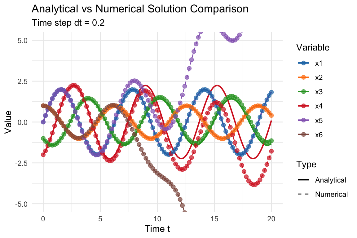
and the general solution in determined without fixing any initial value.
Code
t_max <- 20
dt <- 0.2

# 1. Preparazione dati analitici
t_fine <- seq(0, t_max, length.out = 500)
sol_analitica <- data.frame(
  Time = rep(t_fine, 6),
  Value = c(2*sin(t_fine), cos(t_fine), -sin(t_fine)-cos(t_fine),
            sin(t_fine)-2*cos(t_fine), 2*sin(t_fine), cos(t_fine)),
  Variable = factor(rep(paste0("x", 1:6), each = length(t_fine))),
  Type = "Analytical"
)

# 2. Soluzione numerica
t_numerico <- seq(0, t_max, by = dt)
sistema_ode <- function(t, stato) {
  c(2*cos(t), sin(t)-stato[1], sin(t)-stato[2],
    sin(t)-stato[3], sin(t)-stato[4], sin(t)-stato[5])
}

metodo_heun <- function(f, y0, t_span, h) {
  n <- length(t_span)
  y <- matrix(NA, n, length(y0))
  y[1,] <- y0
  for (i in 2:n) {
    t <- t_span[i-1]
    k1 <- f(t, y[i-1,])
    k2 <- f(t+h, y[i-1,]+h*k1)
    y[i,] <- y[i-1,] + h/2*(k1+k2)
  }
  return(y)
}

sol_numerica <- metodo_heun(sistema_ode, c(0,1,-1,-2,0,1), t_numerico, dt) %>%
  as.data.frame() %>%
  setNames(paste0("x",1:6)) %>%
  mutate(Time = t_numerico, Type = "Numerical") %>%
  pivot_longer(-c(Time,Type), names_to="Variable", values_to="Value")

# 3. Plot combinato
ggplot(bind_rows(sol_analitica, sol_numerica),
       aes(x=Time, y=Value, color=Variable, linetype=Type)) +
  geom_line(data=~filter(.x, Type=="Analytical"), linewidth=0.8) +
  geom_line(data=~filter(.x, Type=="Numerical"), linewidth=0.5) +
  geom_point(data=~filter(.x, Type=="Numerical"), size=2, alpha=0.7) +
  scale_color_manual(values=c("#1f77b4","#ff7f0e","#2ca02c",
                            "#d62728","#9467bd","#8c564b")) +
  scale_linetype_manual(values=c("Analytical"="solid","Numerical"="dashed")) +
  coord_cartesian(ylim=c(-5,5)) +
  labs(title="Analytical vs Numerical Solution Comparison",
       subtitle=paste("Time step dt =", dt),
       x="Time t", y="Value") +
theme_minimal()25.2 Index reduction using dummy variable
Variable classification
- Differential variables: x_1, x_2, x_3, x_4. x_5
- Algebraic variables: x_6
We attempt to solve for u_6 and v_{\text{dot}}, but due to the presence of \lambda, the system is not yet solvable explicitly. We proceed by differentiating.
Step 1: Differentiate algebraic constraints
Differentiate \text{(Constraint 1)} = \cos t-x_6:
\dfrac{\mathrm{d}\text{(Constraint 1)} }{\mathrm{d}t} = -\sin t - x'_6
Substitute known differential variables:
\color{DarkRed}\text{(Constraint 2)} = x_5 - 2\sin t
x'_1 not found, continue index reduction.
Step 2: Differentiate algebraic constraints
Differentiate \text{(Constraint 2)}
\dfrac{\mathrm{d}\text{(Constraint 2)} }{\mathrm{d}t} = x'_5 - 2\cos t \quad\implies\quad \color{DarkRed}\text{(Constraint 3)} = \sin t - 2\cos t - x_4
x'_1 not found, continue index reduction.
Step 3: Differentiate algebraic constraints
Differentiate \text{(Constraint 3)}:
\dfrac{\mathrm{d}\text{(Constraint 3)} }{\mathrm{d}t} = \cos t + 2\sin t - x'_4 \quad\implies\quad \color{DarkRed}\text{(Constraint 4)} = \cos t + \sin t + x_3
x'_1 not found, continue index reduction.
Step 4: Differentiate algebraic constraints
Differentiate \text{(Constraint 4)}:
\dfrac{\mathrm{d}\text{(Constraint 4)}}{\mathrm{d}t} = -\sin t + \cos t + x'_3 \quad\implies\quad \color{DarkRed}\text{(Constraint 5)} = \cos t - x_2
x'_1 not found, continue index reduction.
Step 5: Differentiate algebraic constraints
Differentiate \text{(Constraint 5)}:
\dfrac{\mathrm{d}\text{(Constraint 5)}}{\mathrm{d}t} = -\sin t - x'_2 \quad\implies\quad \color{DarkRed}\text{(Constraint 6)} = -2\sin t + x_1
x'_1 not found, continue index reduction.
Step 6: Differentiate algebraic constraints
Differentiate \text{(Constraint 6)}:
\dfrac{\mathrm{d}\text{(Constraint 6)}}{\mathrm{d}t} = -2\cos t - 2\sin t + x'_1
x'_1 found, index reduction complete
\left\{ \begin{aligned} \color{blue} x_6' &\color{blue}= \sin t - x_5 \\ \color{blue} x_5' &\color{blue}= \sin t - x_4 \\ \color{blue} x_4' &\color{blue}= \sin t - x_3 \\ \color{blue} x_3' &\color{blue}= \sin t - x_2 \\ \color{blue} x_2' &\color{blue}= \sin t - x_1 \\ \color{blue} x_1' &\color{blue}= 2\sin t \end{aligned} \right. \qquad \left\{ \begin{aligned} \color{DarkRed}\text{(Constraint 1)} &\color{DarkRed} = \cos t - x_6 = 0\\ \color{DarkRed}\text{(Constraint 2)} &\color{DarkRed} = x_5 - 2\sin t = 0\\ \color{DarkRed}\text{(Constraint 3)} &\color{DarkRed} = \sin t - 2 \cos t - x_4 = 0\\ \color{DarkRed}\text{(Constraint 4)} &\color{DarkRed} = \sin t + \cos t + x_3 = 0\\ \color{DarkRed}\text{(Constraint 5)} &\color{DarkRed} = \cos t - x_2 = 0\\ \color{DarkRed}\text{(Constraint 6)} &\color{DarkRed} = x_1 -2\sin t = 0 \end{aligned} \right.
Applied 6 time differentiation, the index is 6.
Code
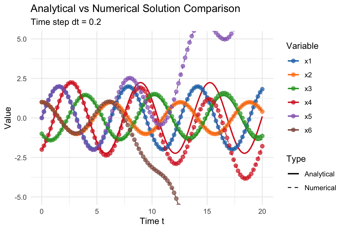
t_max <- 20
dt <- 0.2

# 1. Preparazione dati analitici
t_fine <- seq(0, t_max, length.out = 500)
sol_analitica <- data.frame(
  Time = rep(t_fine, 6),
  Value = c(2*sin(t_fine), cos(t_fine), -sin(t_fine)-cos(t_fine),
            sin(t_fine)-2*cos(t_fine), 2*sin(t_fine), cos(t_fine)),
  Variable = factor(rep(paste0("x", 1:6), each = length(t_fine))),
  Type = "Analytical"
)

# 2. Soluzione numerica
t_numerico <- seq(0, t_max, by = dt)
sistema_ode <- function(t, stato) {
  c(2*cos(t), sin(t)-stato[1], sin(t)-stato[2],
    sin(t)-stato[3], sin(t)-stato[4], sin(t)-stato[5])
}

metodo_heun <- function(f, y0, t_span, h) {
  n <- length(t_span)
  y <- matrix(NA, n, length(y0))
  y[1,] <- y0
  for (i in 2:n) {
    t <- t_span[i-1]
    k1 <- f(t, y[i-1,])
    k2 <- f(t+h, y[i-1,]+h*k1)
    y[i,] <- y[i-1,] + h/2*(k1+k2)
  }
  return(y)
}

sol_numerica <- metodo_heun(sistema_ode, c(0,1,-1,-2,0,1), t_numerico, dt) %>%
  as.data.frame() %>%
  setNames(paste0("x",1:6)) %>%
  mutate(Time = t_numerico, Type = "Numerical") %>%
  pivot_longer(-c(Time,Type), names_to="Variable", values_to="Value")

# 3. Plot combinato
ggplot(bind_rows(sol_analitica, sol_numerica),
       aes(x=Time, y=Value, color=Variable, linetype=Type)) +
  geom_line(data=~filter(.x, Type=="Analytical"), linewidth=0.8) +
  geom_line(data=~filter(.x, Type=="Numerical"), linewidth=0.5) +
  geom_point(data=~filter(.x, Type=="Numerical"), size=2, alpha=0.7) +
  scale_color_manual(values=c("#1f77b4","#ff7f0e","#2ca02c",
                            "#d62728","#9467bd","#8c564b")) +
  scale_linetype_manual(values=c("Analytical"="solid","Numerical"="dashed")) +
  coord_cartesian(ylim=c(-5,5)) +
  labs(title="Analytical vs Numerical Solution Comparison",
       subtitle=paste("Time step dt =", dt),
       x="Time t", y="Value") +
  theme_minimal()